Homework #2 – Getting Started Guide

Spectroscopic Analysis

Note

This section covers essential concepts for working with spectroscopic data, including file formats, peak detection, and visualization techniques.

import numpy as np
from scipy.interpolate import splrep, splev
import matplotlib.pyplot as plt

Standard Scientific Data Formats

Scientific instruments store both measurements and metadata in standardized formats. JCAMP-DX, a common spectroscopy format, illustrates key principles found in ROD files:

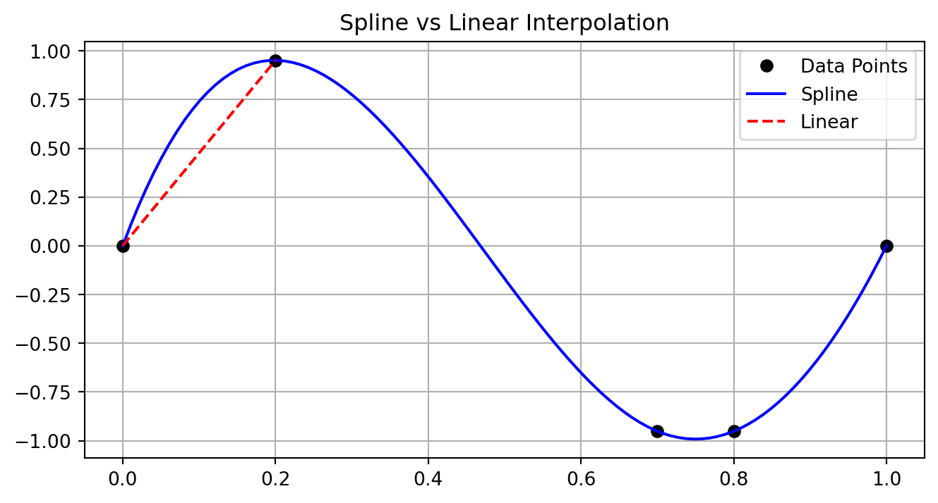
# Example format with metadata and measurements
spectrum = """
##TITLE=Reference Sample
##BLOCKS=1
##XUNITS=1/CM
##YUNITS=ABSORBANCE
##XYDATA=(X++(Y..Y))
500.0  0.033  0.037  0.041
600.0  0.042  0.043  0.044
"""

# Extract data section
for line in spectrum.split('\n'):
    if line.startswith('##'):
        print(f"Metadata: {line}")
    elif line.strip():
        print(f"Data: {line}")

Metadata: ##TITLE=Reference Sample
Metadata: ##BLOCKS=1
Metadata: ##XUNITS=1/CM
Metadata: ##YUNITS=ABSORBANCE
Metadata: ##XYDATA=(X++(Y..Y))
Data: 500.0  0.033  0.037  0.041
Data: 600.0  0.042  0.043  0.044

Spline Interpolation Fundamentals

Cubic splines preserve continuity through second derivatives, essential for peak analysis. Compare with simpler linear interpolation:

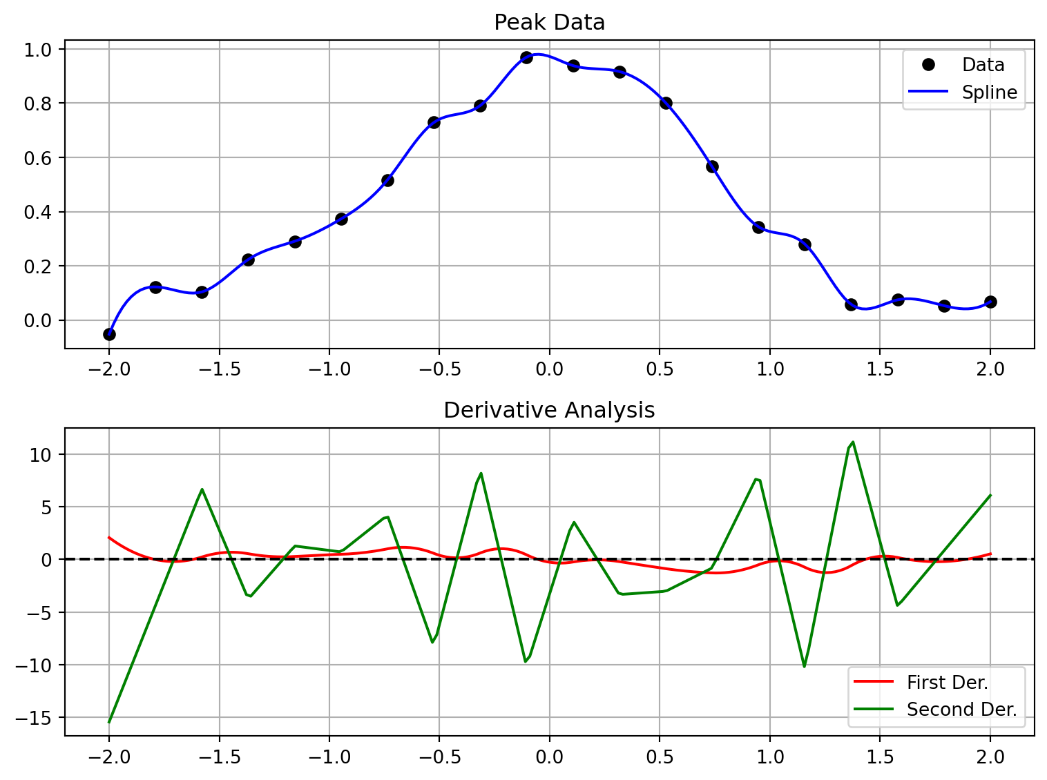
# Generate sparse, uneven samples
x_sparse = np.array([0, 0.2, 0.7, 0.8, 1.0])
y_sparse = np.sin(2*np.pi*x_sparse)

# Fit spline
spl = splrep(x_sparse, y_sparse)
x_dense = np.linspace(0, 1, 100)
y_spline = splev(x_dense, spl)

plt.figure(figsize=(8,4))
plt.plot(x_sparse, y_sparse, 'ko', label='Data Points')
plt.plot(x_dense, y_spline, 'b-', label='Spline')
plt.plot([x_sparse[0], x_sparse[1]], [y_sparse[0], y_sparse[1]], 
         'r--', label='Linear')
plt.grid(True)
plt.legend()
plt.title('Spline vs Linear Interpolation')
plt.show()

Critical Points and Derivatives

First derivatives identify maxima (zero crossings), while second derivatives characterize peak shapes:

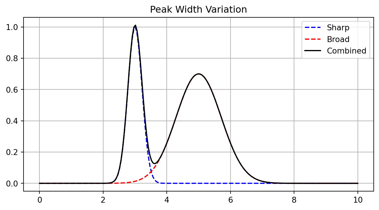
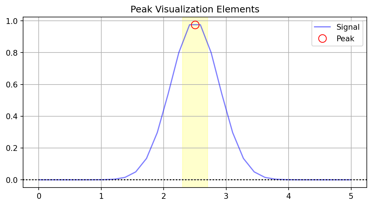
# Generate example peak
x = np.linspace(-2, 2, 20)
y = np.exp(-x**2) + 0.05*np.random.randn(len(x))

# Fit and compute derivatives
spl = splrep(x, y)
x_fine = np.linspace(-2, 2, 200)
y_smooth = splev(x_fine, spl)
dy = splev(x_fine, spl, der=1)
d2y = splev(x_fine, spl, der=2)

fig, (ax1, ax2) = plt.subplots(2, 1, figsize=(8,6))
# Original and smoothed data
ax1.plot(x, y, 'ko', label='Data')
ax1.plot(x_fine, y_smooth, 'b-', label='Spline')
ax1.grid(True)
ax1.legend()
ax1.set_title('Peak Data')

# Derivatives
ax2.plot(x_fine, dy, 'r-', label='First Der.')
ax2.plot(x_fine, d2y, 'g-', label='Second Der.')
ax2.axhline(y=0, color='k', linestyle='--')
ax2.grid(True)
ax2.legend()
ax2.set_title('Derivative Analysis')
plt.tight_layout()
plt.show()

Spectral Peak Characteristics

Molecular spectra exhibit peaks with varying widths and intensities:

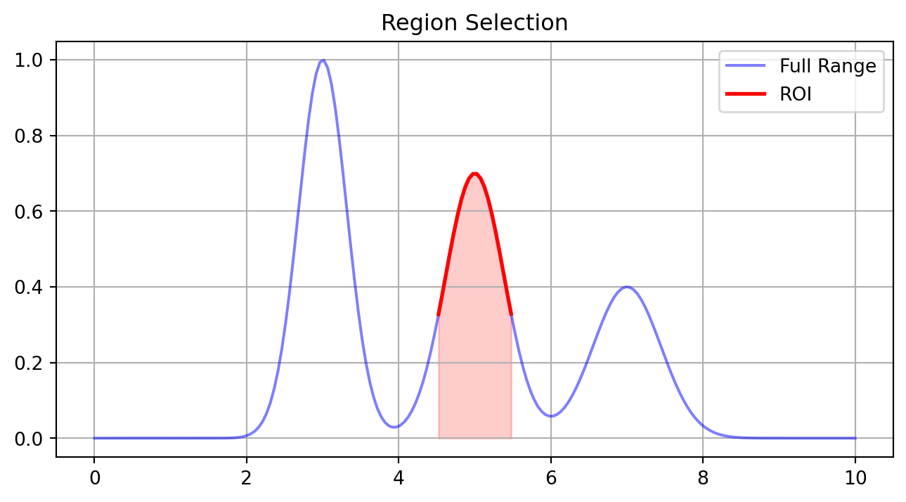
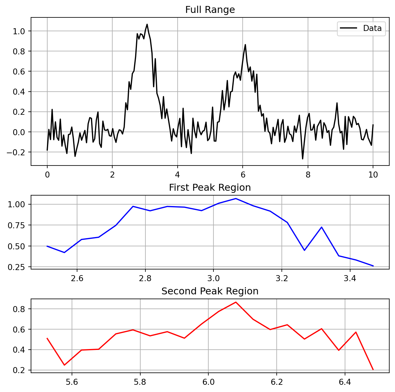
# Generate peaks with different properties
x = np.linspace(0, 10, 200)
sharp = np.exp(-(x-3)**2/0.1)    # Narrow peak
broad = 0.7*np.exp(-(x-5)**2/1.0) # Wide peak
combo = sharp + broad

plt.figure(figsize=(8,4))
plt.plot(x, sharp, 'b--', label='Sharp')
plt.plot(x, broad, 'r--', label='Broad')
plt.plot(x, combo, 'k-', label='Combined')
plt.grid(True)
plt.legend()
plt.title('Peak Width Variation')
plt.show()

Region of Interest Analysis

Focused analysis requires careful region selection:

# Generate data with multiple features
x = np.linspace(0, 10, 200)
y = (np.exp(-(x-3)**2/0.2) + 
     0.7*np.exp(-(x-5)**2/0.3) +
     0.4*np.exp(-(x-7)**2/0.4))

# Analyze specific region
region = (x >= 4.5) & (x <= 5.5)
x_roi = x[region]
y_roi = y[region]

plt.figure(figsize=(8,4))
plt.plot(x, y, 'b-', label='Full Range', alpha=0.5)
plt.plot(x_roi, y_roi, 'r-', label='ROI', linewidth=2)
plt.fill_between(x_roi, y_roi, alpha=0.2, color='red')
plt.grid(True)
plt.legend()
plt.title('Region Selection')
plt.show()

Plot Styling for Peak Analysis

Clear peak visualization requires appropriate styling:

x_demo = np.linspace(0, 5, 30)
y_demo = np.exp(-(x_demo-2.5)**2/0.3)

plt.figure(figsize=(8,4))
# Base data
plt.plot(x_demo, y_demo, 'b-', label='Signal', alpha=0.5)
# Peak marker
plt.plot(2.5, np.max(y_demo), 'ro', markersize=10, 
         markerfacecolor='none', label='Peak')
# Baseline
plt.axhline(y=0, color='k', linestyle=':')
# Region highlight
plt.axvspan(2.3, 2.7, color='yellow', alpha=0.2)

plt.grid(True)
plt.legend()
plt.title('Peak Visualization Elements')
plt.show()

Error Handling Patterns

Robust data processing requires careful validation:

def validate_spectrum(x, y):
    """Example validation checks"""
    if len(x) != len(y):
        return False, "Length mismatch"
    if not all(x[i] <= x[i+1] for i in range(len(x)-1)):
        return False, "X values not monotonic"
    if any(np.isnan(y)):
        return False, "Contains NaN values"
    return True, "Valid spectrum"

# Test cases
x_test = np.array([1, 2, 3, 2])
y_test = np.array([0.1, 0.2, 0.3, 0.4])
print(validate_spectrum(x_test, y_test))

(False, 'X values not monotonic')

Multi-Panel Visualization

Complex analysis requires multiple linked views:

# Generate example spectrum
x = np.linspace(0, 10, 200)
y = (np.exp(-(x-3)**2/0.2) + 
     0.7*np.exp(-(x-6)**2/0.3) +
     0.1*np.random.randn(len(x)))

# Create multi-panel figure
fig = plt.figure(figsize=(8,8))
gs = fig.add_gridspec(3, 1, height_ratios=[2,1,1], hspace=0.3)

# Full spectrum
ax1 = fig.add_subplot(gs[0])
ax1.plot(x, y, 'k-', label='Data')
ax1.grid(True)
ax1.legend()
ax1.set_title('Full Range')

# First zoom region
ax2 = fig.add_subplot(gs[1])
mask1 = (x >= 2.5) & (x <= 3.5)
ax2.plot(x[mask1], y[mask1], 'b-')
ax2.grid(True)
ax2.set_title('First Peak Region')

# Second zoom region
ax3 = fig.add_subplot(gs[2])
mask2 = (x >= 5.5) & (x <= 6.5)
ax3.plot(x[mask2], y[mask2], 'r-')
ax3.grid(True)
ax3.set_title('Second Peak Region')

plt.show()

The Ising Model

Note

The Ising model demonstrates how complex physical behavior emerges from simple rules. This section covers implementation aspects of Monte Carlo simulation.

The Ising Model and Monte Carlo Methods

The Ising model represents one of physics’ most successful simplified models, capturing complex collective behavior from simple local interactions.

Physical Foundations

The model assigns binary spins (\(s_i \in \{-1,+1\}\)) to lattice sites. The energy depends on nearest-neighbor interactions:

\(E = -J\sum_{\langle i,j \rangle} s_i s_j\)

where \(J\) is the coupling constant (typically set to 1) and \(\langle i,j \rangle\) denotes summation over nearest neighbors.

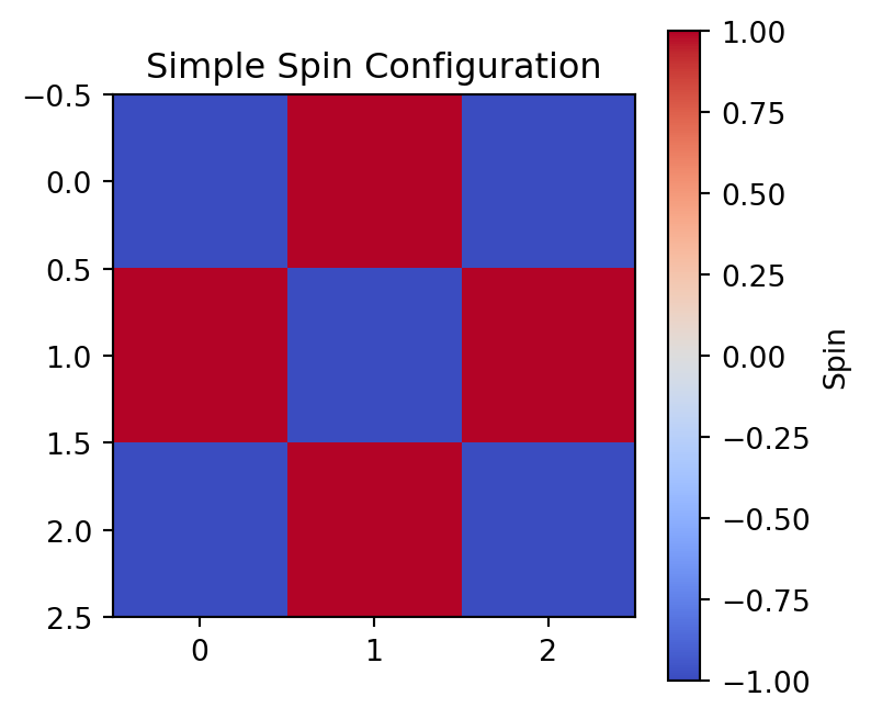
import numpy as np
import matplotlib.pyplot as plt

# Nearest neighbor, Ising
grid = np.array([
    [-1,  1, -1],
    [ 1, -1,  1],
    [-1,  1, -1]
])

plt.figure(figsize=(4,4))
plt.imshow(grid, cmap='coolwarm')
plt.colorbar(label='Spin')
plt.title('Simple Spin Configuration')
plt.show()

# Energy calculation for center spin
i, j = 1, 1
center = grid[i,j]
neighbors = (grid[i-1,j] + grid[i+1,j] + 
            grid[i,j-1] + grid[i,j+1])
E_center = -center * neighbors
print(f"Energy contribution from center: {E_center}")

Energy contribution from center: 4

Phase Transitions

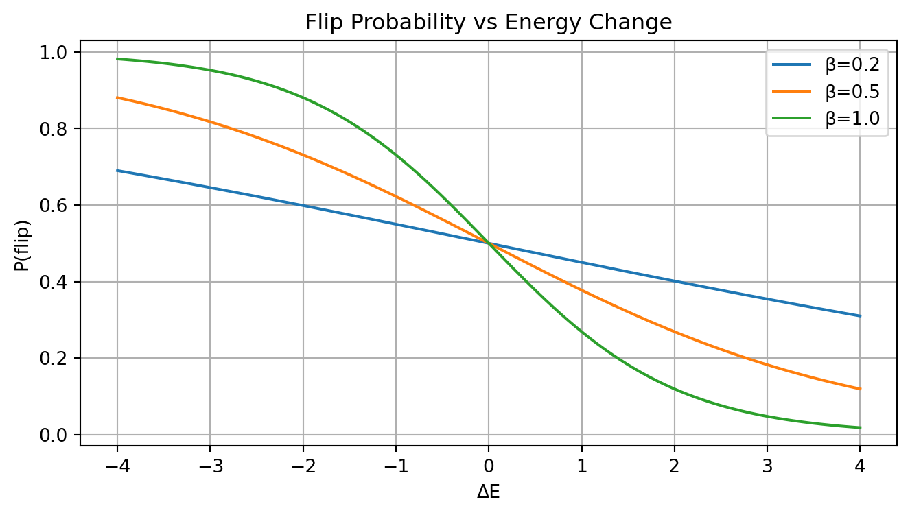
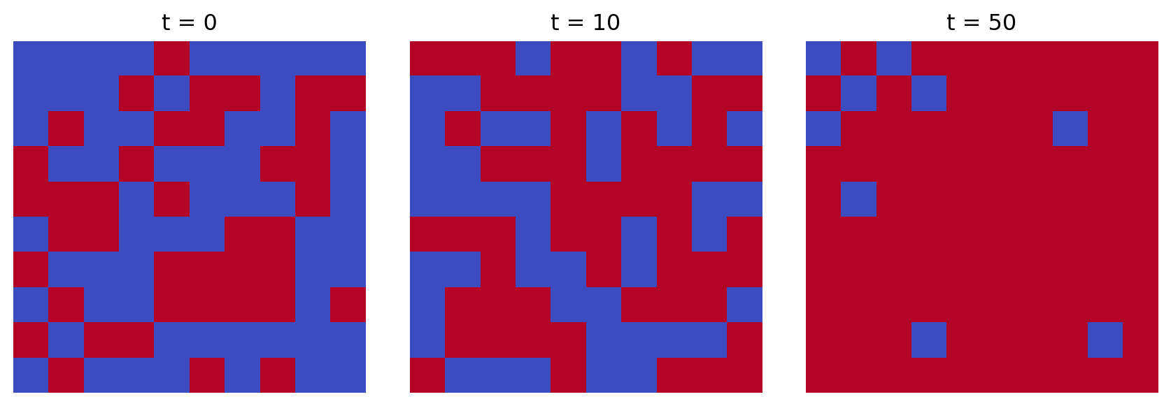
The Ising model exhibits a phase transition between ordered (low temperature) and disordered (high temperature) states. The inverse temperature β controls this behavior:

\(P(\text{flip}) = \frac{1}{1 + e^{\beta \Delta E}}\)

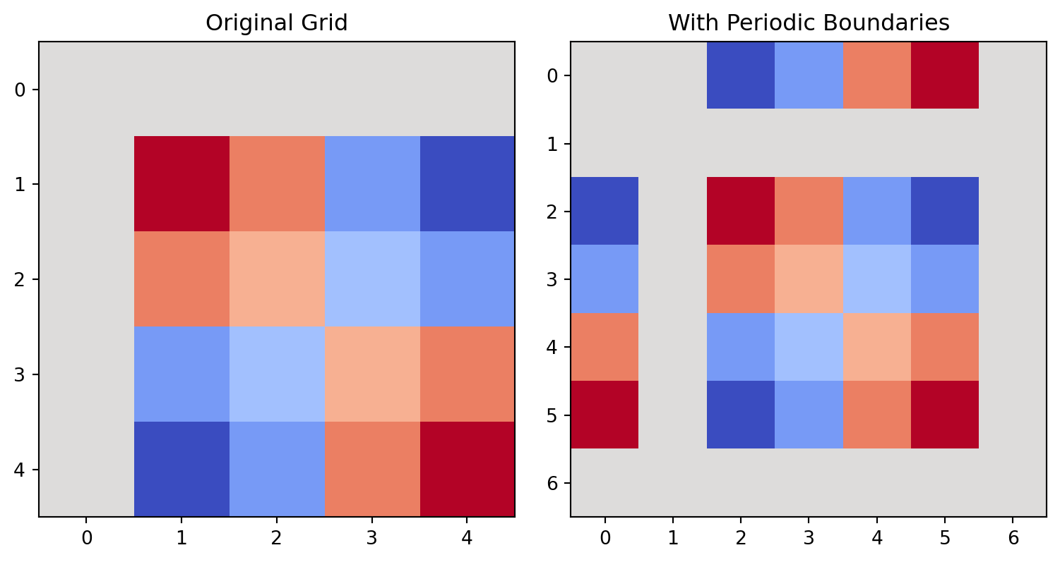
# Visualize flip probability
dE = np.linspace(-4, 4, 100)
betas = [0.2, 0.5, 1.0]

plt.figure(figsize=(8,4))
for beta in betas:
    P = 1/(1 + np.exp(beta * dE))
    plt.plot(dE, P, label=f'β={beta}')
    
plt.grid(True)
plt.xlabel('ΔE')
plt.ylabel('P(flip)')
plt.title('Flip Probability vs Energy Change')
plt.legend()
plt.show()

Periodic Boundary Conditions

Periodic boundaries minimize edge effects by wrapping the lattice:

def show_periodic(N=5):
    # Generate simple pattern
    x = np.arange(N)
    y = np.arange(N)
    X, Y = np.meshgrid(x, y)
    pattern = np.sin(2*np.pi*X/N) * np.sin(2*np.pi*Y/N)
    
    plt.figure(figsize=(8,4))
    
    # Original
    plt.subplot(121)
    plt.imshow(pattern, cmap='coolwarm')
    plt.title('Original Grid')
    
    # With periodic extension
    extended = np.zeros((N+2, N+2))
    extended[1:-1, 1:-1] = pattern
    # Add periodic boundaries
    extended[0, 1:-1] = pattern[-1, :]  # Top
    extended[-1, 1:-1] = pattern[0, :]  # Bottom
    extended[1:-1, 0] = pattern[:, -1]  # Left
    extended[1:-1, -1] = pattern[:, 0]  # Right
    
    plt.subplot(122)
    plt.imshow(extended, cmap='coolwarm')
    plt.title('With Periodic Boundaries')
    
    plt.tight_layout()
    plt.show()

show_periodic()

Energy Updates

Local energy changes can be computed efficiently:

def energy_change_example(grid, i, j):
    """energy change calculation"""
    N = len(grid)
    current_spin = grid[i,j]
    # Get neighbors with periodic boundaries
    neighbors = (grid[(i+1)%N, j] + grid[i-1, j] +
                grid[i, (j+1)%N] + grid[i, (j-1)%N])
    
    # Energy before and after flip
    E_before = -current_spin * neighbors
    E_after = current_spin * neighbors  # Flipped spin
    return E_after - E_before

# Example grid
N = 4
grid = np.random.choice([-1, 1], size=(N,N))
i, j = 1, 1
dE = energy_change_example(grid, i, j)
print(f"Energy change for flip at ({i},{j}): {dE}")

Energy change for flip at (1,1): 0

Magnetization Evolution

The average magnetization \(M = \frac{1}{N^2}\sum_{i,j} s_{ij}\) serves as an order parameter:

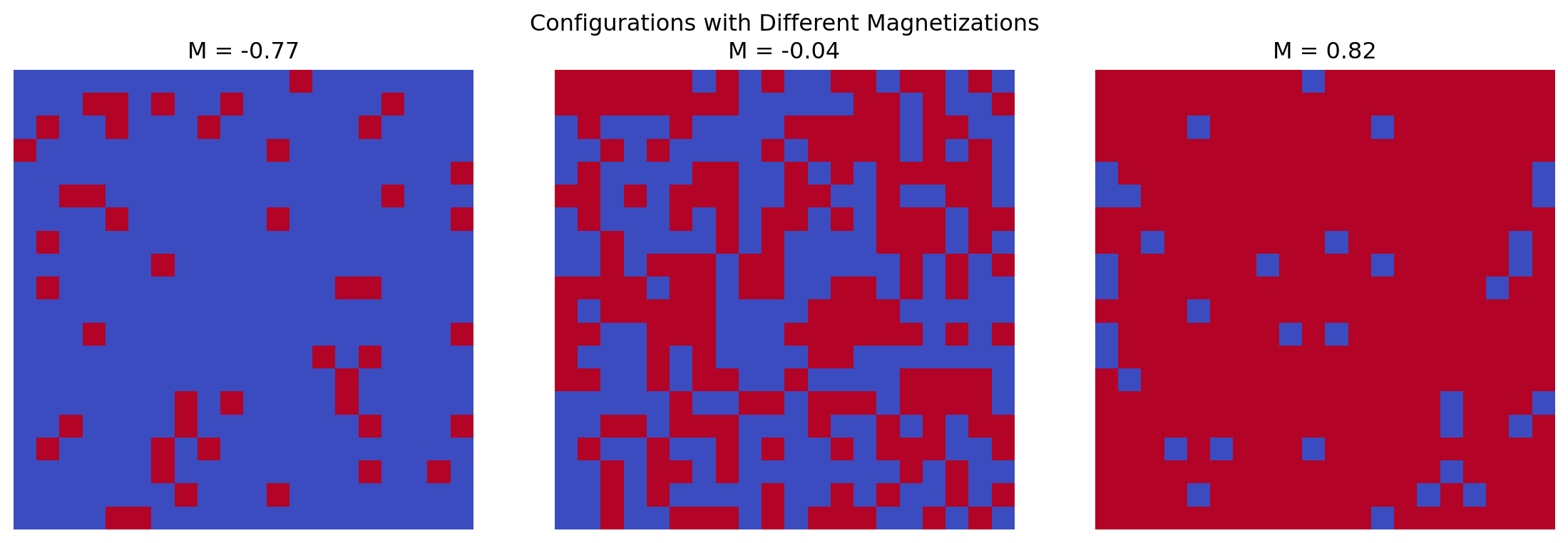
# magnetization calculation
def calculate_magnetization(grid):
    return np.mean(grid)

# Generate random configurations at different "temperatures"
N = 20
n_configs = 3
fig, axes = plt.subplots(1, n_configs, figsize=(12,4))

for i, p in enumerate([0.1, 0.5, 0.9]):
    # p controls bias towards +1
    grid = np.random.choice([-1, 1], size=(N,N), p=[1-p, p])
    m = calculate_magnetization(grid)
    
    axes[i].imshow(grid, cmap='coolwarm')
    axes[i].set_title(f'M = {m:.2f}')
    axes[i].axis('off')

plt.suptitle('Configurations with Different Magnetizations')
plt.tight_layout()
plt.show()

State Visualization

Effective visualization helps track system evolution:

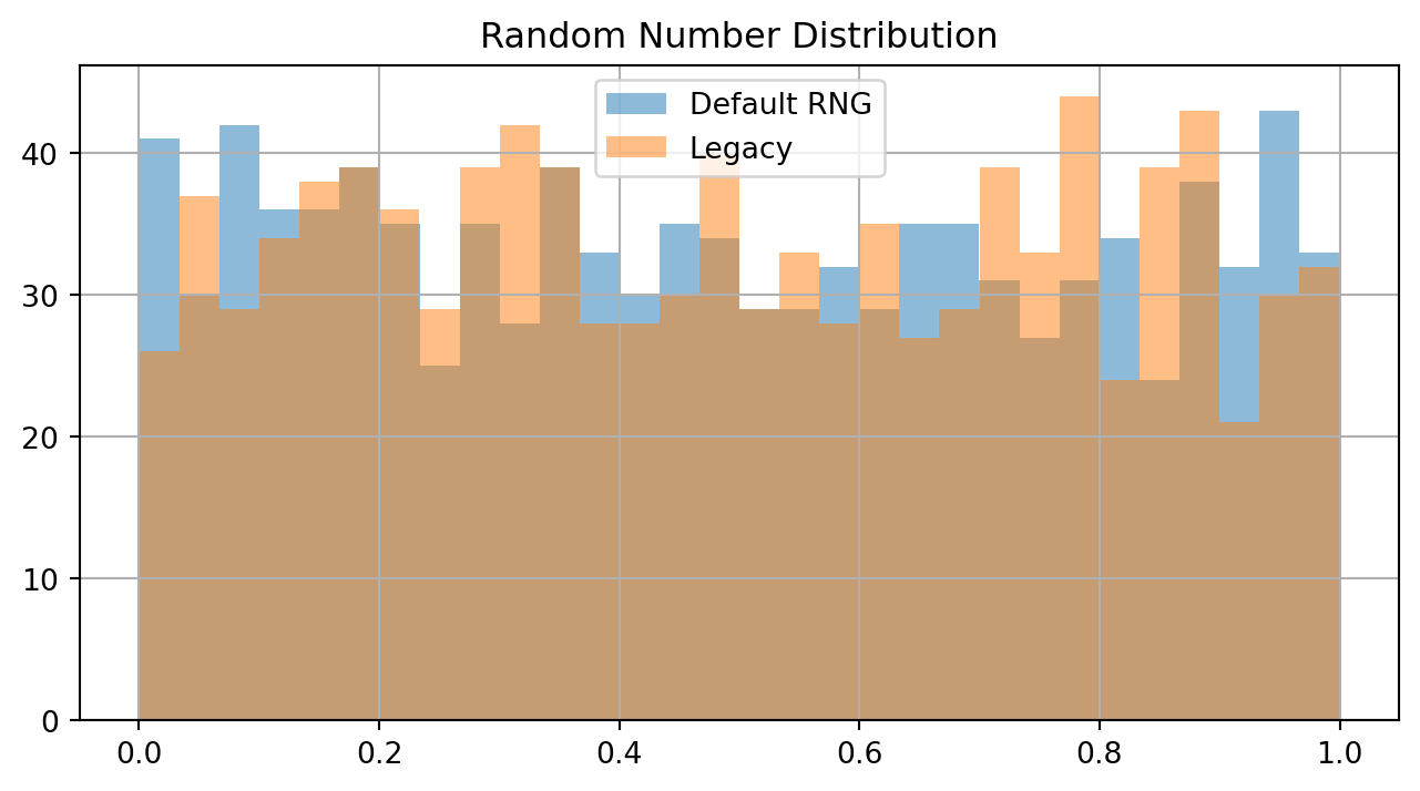
def plot_state_evolution(states, times):
    """Plot grid states at different times"""
    n = len(times)
    fig, axes = plt.subplots(1, n, figsize=(3*n, 3))
    
    for ax, state, t in zip(axes, states, times):
        ax.imshow(state, cmap='coolwarm')
        ax.set_title(f't = {t}')
        ax.axis('off')
    
    plt.tight_layout()
    plt.show()

# Generate example evolution
N = 10
states = []
times = [0, 10, 50]
for t in times:
    # Simulate different stages of ordering
    p = min(0.5 + t/100, 0.9)
    state = np.random.choice([-1, 1], size=(N,N), p=[1-p, p])
    states.append(state)

plot_state_evolution(states, times)

Random Number Generation

The quality of random numbers affects simulation results:

# Compare random number generators
n_samples = 1000
rng = np.random.default_rng()  # Newer generator
rand1 = rng.random(n_samples)
rand2 = np.random.rand(n_samples)  # Legacy

plt.figure(figsize=(8,4))
plt.hist(rand1, bins=30, alpha=0.5, label='Default RNG')
plt.hist(rand2, bins=30, alpha=0.5, label='Legacy')
plt.grid(True)
plt.legend()
plt.title('Random Number Distribution')
plt.show()

Command Line Applications

Note

Building robust command-line applications requires careful handling of input validation, error cases, and program output. This section shows key patterns.

Command-Line Numerical Methods

Root Finding Context

The secant method approximates roots through successive linear interpolation:

\(x_{n+1} = x_n - f(x_n)\frac{x_n - x_{n-1}}{f(x_n) - f(x_{n-1})}\)

Unlike Newton’s method, it avoids derivative calculations but requires two initial points.

Command-Line Argument Processing

Python’s sys.argv provides command-line arguments as strings:

import sys

# Example command: python script.py 1.1 1.4
def parse_args():
    try:
        # Skip script name (argv[0])
        args = sys.argv[1:]
        if len(args) != 2:
            print("Usage: script.py a b", file=sys.stderr)
            return
            
        print(f"Arguments received: {args}")
    except Exception as e:
        print(f"Error: {str(e)}", file=sys.stderr)

Type Conversion and Validation

Convert and validate string inputs to appropriate types:

def validate_numeric(value_str):
    try:
        return float(value_str)
    except ValueError:
        raise ValueError(f"'{value_str}' is not numeric")

# Example usage
test_values = ["1.23", "abc", "2.5"]
for val in test_values:
    try:
        num = validate_numeric(val)
        print(f"Converted {val} to {num}")
    except ValueError as e:
        print(f"Error: {e}")

Converted 1.23 to 1.23
Error: 'abc' is not numeric
Converted 2.5 to 2.5

Error Stream vs Output Stream

Python provides separate streams for normal output and errors:

import sys

def output_streams():
    # Normal output goes to stdout
    print("Processing data...")
    
    # Errors and warnings go to stderr
    print("Warning: value out of range", file=sys.stderr)

# Usage example
output_streams()

Processing data...

Warning: value out of range

Function Import Patterns

Importing external functions requires careful path handling:

import os
import sys

# Add current directory to path
sys.path.append(os.path.abspath('.'))

# Import function from module
try:
    from func import f
except ImportError:
    print("Error: Cannot import function", file=sys.stderr)
    sys.exit(1)

Bracket Validation

Root bracketing requires checking signs:

import math

def check_bracket(f, a, b):
    """Verify root bracketing using Bolzano's theorem"""
    try:
        fa, fb = f(a), f(b)
        if fa * fb >= 0:
            return False, "Values don't bracket root"
        return True, "Valid bracket"
    except Exception as e:
        return False, f"Evaluation error: {str(e)}"

# Example with cos(x)
f = math.cos
print(check_bracket(f, 0, math.pi/2))  # No root
print(check_bracket(f, 0, math.pi))    # Contains root

(False, "Values don't bracket root")
(True, 'Valid bracket')

Precision and Formatting

Control numeric output precision:

x = 1.23456789
# Various formatting options
print(f"{x:.6f}")   # Fixed precision
print(f"{x:.2e}")   # Scientific
print(f"{x:.20f}")  # High precision

1.234568
1.23e+00
1.23456788999999989009

Exception Handling Patterns

Structure try-except blocks for clarity:

def process_value(x):
    try:
        # Main operation block
        result = float(x)
        
    except ValueError:
        # Handle type conversion
        print("Invalid number format", file=sys.stderr)
        return None
        
    except ZeroDivisionError:
        # Handle computational error
        print("Division by zero", file=sys.stderr)
        return None
        
    except Exception as e:
        # Catch unexpected errors
        print(f"Unexpected error: {e}", file=sys.stderr)
        return None
        
    return result

Exit Codes and Status

Proper program termination with status:

import sys

def main():
    try:
        # Main program logic
        process_data()
        return 0  # Success
        
    except ValueError:
        print("Invalid input", file=sys.stderr)
        return 1  # Error code
        
    except Exception as e:
        print(f"Error: {e}", file=sys.stderr)
        return 2  # Different error code

if __name__ == "__main__":
    sys.exit(main())