Homework #5 – Getting Started Guide

1 Logistic Regression and the MNIST Dataset

1.1 Binary Classification with Logistic Regression

Logistic regression extends linear models to classification by applying a nonlinear transformation to the output. For logistic regression specifically, this transformation maps the linear predictor to conditional probabilities \(P(Y=1|X)\) between 0 and 1, providing a probabilistic framework for making binary decisions.

1.1.1 The Sigmoid Function as a Nonlinear Detector

The logistic (sigmoid) function transforms any real-valued input into the range (0,1):

\[\sigma(z) = \frac{1}{1 + e^{-z}}\]

This transformation functions as a soft threshold detector. The function’s gradient provides critical information about sensitivity to input changes:

\[\frac{d\sigma}{dz} = \sigma(z)(1-\sigma(z))\]

The gradient reaches its maximum value of 0.25 at z=0 (where \(\sigma(z)=0.5\)), making the function most sensitive precisely at the decision boundary. This mathematical property is fundamental to the learning process in logistic regression.

Code
def sigmoid(z):
    """Numerically stable implementation of sigmoid function"""
    return np.where(z >= 0, 
                  1 / (1 + np.exp(-z)),
                  np.exp(z) / (1 + np.exp(z)))

def sigmoid_derivative(z):
    """Derivative of the sigmoid function"""
    s = sigmoid(z)
    return s * (1 - s)

# Visualize sigmoid and its derivative
z = np.linspace(-6, 6, 100)
sig = sigmoid(z)
dsig = sigmoid_derivative(z)

# Plot sigmoid and derivative
plt.figure(figsize=(10, 5))
plt.plot(z, sig, 'b-', linewidth=2, label='Sigmoid function')
plt.plot(z, dsig, 'r-', linewidth=2, label='Derivative')

# Illustrate tangent line at a specific point
point_z = 2
point_s = sigmoid(point_z)
point_d = sigmoid_derivative(point_z)

# Mark the point
plt.plot(point_z, point_s, 'ko', markersize=8)

# Draw tangent line
x_tangent = np.array([point_z - 2, point_z + 2])
y_tangent = point_s + point_d * (x_tangent - point_z)
plt.plot(x_tangent, y_tangent, 'g--', linewidth=2, 
         label=f'Tangent at z={point_z}, slope={point_d:.3f}')

plt.grid(True)
plt.legend()
plt.title('Sigmoid Function and Its Derivative')
plt.xlabel('z')
plt.ylabel('σ(z)')
plt.axhline(y=0, color='k', linestyle='-', alpha=0.3)
plt.axhline(y=1, color='k', linestyle='-', alpha=0.3)
plt.axvline(x=0, color='k', linestyle='-', alpha=0.3)

Sigmoid function with derivative and tangent line

The forward propagation in logistic regression combines the linear model with the sigmoid function:

Code
def predict_proba(X, w, b):
    """
    Forward propagation for logistic regression
    
    Parameters:
    X: input features matrix (n_samples, n_features)
    w: weight vector (n_features,)
    b: bias term (scalar)
    
    Returns:
    Predicted probabilities for class 1
    """
    z = X @ w + b
    return sigmoid(z)

1.1.2 Binary Cross-Entropy Loss

Binary cross-entropy loss has foundations in information theory and maximum likelihood estimation:

\[\mathcal{L}(w) = -\frac{1}{N}\sum_{i=1}^{N}[y_i\log(p(x_i)) + (1-y_i)\log(1-p(x_i))]\]

This loss function comes directly from maximum likelihood estimation. When modeling p(x) as the probability that y=1 given model parameters w, the likelihood of our dataset is:

\[L(w) = \prod_{i=1}^{N} p(x_i)^{y_i} (1-p(x_i))^{1-y_i}\]

Taking the negative logarithm yields the binary cross-entropy loss. This direct derivation from probability theory makes binary cross-entropy the mathematically optimal loss function for logistic regression.

Code
def binary_cross_entropy(y_true, y_pred):
    """
    Compute binary cross-entropy loss with numerical stability
    
    Parameters:
    y_true: True binary labels (0 or 1)
    y_pred: Predicted probabilities for class 1
    
    Returns:
    Average binary cross-entropy loss
    """
    epsilon = 1e-15  # Prevent log(0)
    y_pred = np.clip(y_pred, epsilon, 1 - epsilon)
    return -np.mean(y_true * np.log(y_pred) + (1 - y_true) * np.log(1 - y_pred))

1.2 Regularization

Regularization imposes constraints on the system response (weights) to prevent high-gain solutions that would amplify noise in the input data.

1.2.1 L2 Regularization (Ridge)

\[\mathcal{L}_{L2}(w) = \mathcal{L}(w) + \lambda\|w\|_2^2\]

L2 regularization applies a quadratic penalty on weights, analogous to energy constraints in signal processing. It produces a smoother decision boundary by limiting the energy in the weight vector. From a Bayesian perspective, this represents a Gaussian prior on the weights.

1.2.2 L1 Regularization (Lasso)

\[\mathcal{L}_{L1}(w) = \mathcal{L}(w) + \lambda\|w\|_1\]

L1 regularization promotes sparsity in the weight vector, similar to compressed sensing in signal reconstruction. It enforces a constraint that drives many weights to precisely zero, effectively performing feature selection by identifying the most salient pixels for detecting the target digit.

1.2.3 L1 vs L2 Regularization: Geometric Interpretation

Code
from matplotlib.patches import Circle

# Create geometric visualization of L1 vs L2 regularization
fig, ax = plt.subplots(1, 2, figsize=(12, 5))

# Set up centered coordinates
x = np.linspace(-2, 2, 100)
y = np.linspace(-2, 2, 100)
X, Y = np.meshgrid(x, y)

# True optimal point shifted from origin to show tradeoff
# Modified to be not at 45 degrees from origin for better visualization
optimal_point = np.array([1.2, 0.6])  # Intentionally asymmetric

# Standard loss function (elliptical to avoid 45-degree symmetry)
Z_loss = 2*(X-optimal_point[0])**2 + (Y-optimal_point[1])**2

# Contour levels for loss function
loss_levels = np.array([0.2, 0.5, 1.0, 2.0, 3.0])

# Regularization constraint values
l2_constraint = 0.8  # Radius of circle for L2
l1_constraint = 0.8  # Radius of diamond for L1

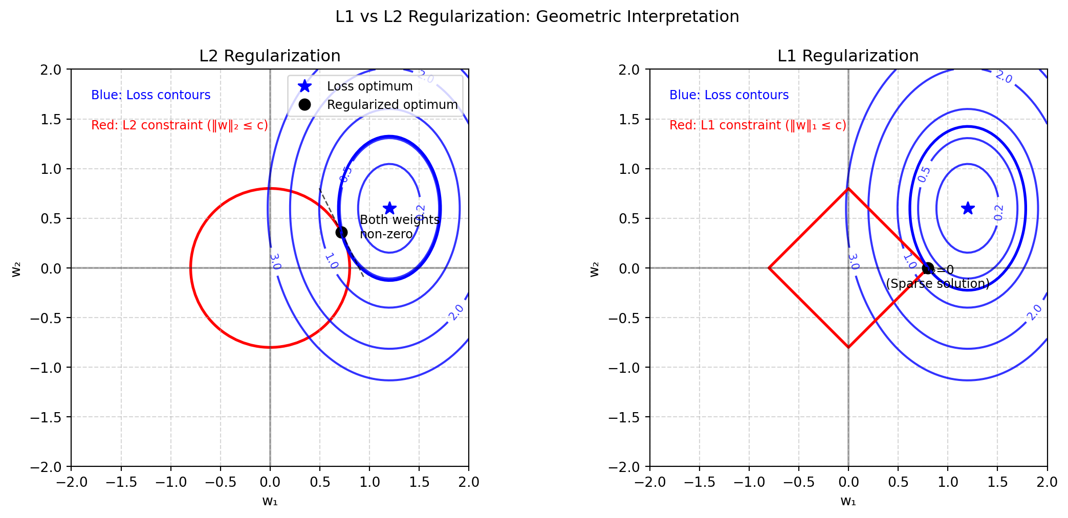
# L2 regularization plot
cs0 = ax[0].contour(X, Y, Z_loss, loss_levels, colors='blue', alpha=0.8, linestyles='-')
l2_circle = Circle((0, 0), l2_constraint, fill=False, color='red', 
                  linestyle='-', linewidth=2)
ax[0].add_patch(l2_circle)

# L1 regularization plot
cs1 = ax[1].contour(X, Y, Z_loss, loss_levels, colors='blue', alpha=0.8, linestyles='-')

# L1 diamond shape
l1_points = np.array([
    [l1_constraint, 0], [0, l1_constraint], 
    [-l1_constraint, 0], [0, -l1_constraint], [l1_constraint, 0]
])
ax[1].plot(l1_points[:,0], l1_points[:,1], 'r-', linewidth=2)

# Mark the true optimal point (standard loss only)
for a in ax:
    a.plot(optimal_point[0], optimal_point[1], 'b*', markersize=10, label='Loss optimum')

# Analytically determine the constrained optimal points
# For L2: Point on circle closest to optimal point (projection)
l2_direction = optimal_point / np.linalg.norm(optimal_point)  # Unit vector toward optimal
l2_optimal = l2_constraint * l2_direction  # Scale to lie on circle

# For L1: Point on diamond closest to optimal point
# Due to the asymmetric loss, the optimal point will be on the x-axis
l1_optimal = np.array([l1_constraint, 0])  # Sparse solution with w₂=0

# Plot optimal points
ax[0].plot(l2_optimal[0], l2_optimal[1], 'ko', markersize=8, label='Regularized optimum')
ax[1].plot(l1_optimal[0], l1_optimal[1], 'ko', markersize=8, label='Regularized optimum')

# Calculate loss at optimal points
l2_loss_value = 2*(l2_optimal[0]-optimal_point[0])**2 + (l2_optimal[1]-optimal_point[1])**2
l1_loss_value = 2*(l1_optimal[0]-optimal_point[0])**2 + (l1_optimal[1]-optimal_point[1])**2

# Add custom contours for the exact loss values at optimal points
ax[0].contour(X, Y, Z_loss, [l2_loss_value], colors='blue', linewidths=2)
ax[1].contour(X, Y, Z_loss, [l1_loss_value], colors='blue', linewidths=2)

# Add contour labels
plt.clabel(cs0, inline=1, fontsize=8, fmt='%.1f')
plt.clabel(cs1, inline=1, fontsize=8, fmt='%.1f')

# Labels and formatting
ax[0].set_title('L2 Regularization')
ax[0].text(-1.8, 1.7, 'Blue: Loss contours', color='blue', fontsize=9)
ax[0].text(-1.8, 1.4, 'Red: L2 constraint (‖w‖₂ ≤ c)', color='red', fontsize=9)
ax[0].text(0.9, 0.3, 'Both weights\nnon-zero', color='black', fontsize=9)
ax[0].legend(loc='upper right', fontsize=9)

ax[1].set_title('L1 Regularization')
ax[1].text(-1.8, 1.7, 'Blue: Loss contours', color='blue', fontsize=9)
ax[1].text(-1.8, 1.4, 'Red: L1 constraint (‖w‖₁ ≤ c)', color='red', fontsize=9)
ax[1].text(l1_constraint + 0.1, -0.2, 'w₂=0\n(Sparse solution)', color='black', ha='center', fontsize=9)

# Draw tangent lines at optimal points to emphasize tangency
def get_tangent_points(center, radius, point):
    # Get two points on tangent line through optimal point
    dx, dy = point[0] - center[0], point[1] - center[1]
    norm = np.sqrt(dx**2 + dy**2)
    nx, ny = -dy/norm, dx/norm  # Normal vector
    return [[point[0] - nx*0.5, point[1] - ny*0.5], 
            [point[0] + nx*0.5, point[1] + ny*0.5]]

# Add tangent line for L2
tangent_l2 = get_tangent_points([0, 0], l2_constraint, l2_optimal)
ax[0].plot([tangent_l2[0][0], tangent_l2[1][0]], 
           [tangent_l2[0][1], tangent_l2[1][1]], 
           'k--', linewidth=1, alpha=0.7)

# Set equal axes limits for better comparison
for a in ax:
    a.set_xlim(-2, 2)
    a.set_ylim(-2, 2)
    a.grid(True, linestyle='--', alpha=0.5)
    a.set_xlabel('w₁')
    a.set_ylabel('w₂')
    a.axhline(y=0, color='k', linestyle='-', alpha=0.3)
    a.axvline(x=0, color='k', linestyle='-', alpha=0.3)
    a.set_aspect('equal')  # Equal aspect ratio

plt.tight_layout()
plt.suptitle('L1 vs L2 Regularization: Geometric Interpretation', y=1.05)
Text(0.5, 1.05, 'L1 vs L2 Regularization: Geometric Interpretation')

Geometric comparison of L1 and L2 regularization constraints

The figure illustrates the geometric difference between L1 and L2 regularization constraints:

  • Left (L2): The circular constraint tangentially intersects the loss contour at a point where both weights are non-zero. The smooth boundary of the L2 constraint rarely coincides with coordinate axes.

  • Right (L1): The diamond-shaped constraint touches the loss contour precisely at a vertex on the w₁ axis (w₂=0). The corners of the L1 constraint align with coordinate axes, promoting sparse solutions.

For MNIST classification, L1 regularization yields sparse solutions where many pixel weights equal zero, effectively performing feature selection. L2 regularization shrinks all weights but rarely nullifies them completely.

1.2.4 Regularization as Bayesian Priors

From a Bayesian perspective, regularization terms correspond directly to prior distributions on model weights. This connection provides additional insight into why different regularization methods produce different behaviors.

In Bayesian inference, we seek to estimate the posterior distribution of weights given the data:

\[p(w|y) = \frac{p(y|w)p(w)}{p(y)}\]

Where \(p(y|w)\) is the likelihood of observing the data given the weights, and \(p(w)\) is the prior probability of the weights. Taking the negative logarithm of the posterior (and dropping the constant denominator), we get:

\[-\log p(w|y) = -\log p(y|w) - \log p(w)\]

For logistic regression with a binary cross-entropy loss function, the negative log-likelihood term is:

\[-\log p(y|w) = \sum_{i=1}^{N}[-y_i\log(p(x_i)) - (1-y_i)\log(1-p(x_i))] = \mathcal{L}(w)\]

The regularization term arises from our prior assumptions about the weights. Consider two common prior distributions:

  1. Gaussian (Normal) Prior: When we assume weights are normally distributed around zero:

    \[p(w) = \prod_{j=1}^{d} \frac{1}{\sqrt{2\pi\sigma^2}} \exp\left(-\frac{w_j^2}{2\sigma^2}\right)\]

    Taking the negative logarithm:

    \[-\log p(w) = \frac{1}{2\sigma^2}\sum_{j=1}^{d} w_j^2 + \text{const} = \frac{\lambda}{2}||w||_2^2 + \text{const}\]

    Where \(\lambda = 1/\sigma^2\). This gives us the L2 regularization term.

  2. Laplace Prior: When we assume weights follow a Laplace distribution:

    \[p(w) = \prod_{j=1}^{d} \frac{1}{2b} \exp\left(-\frac{|w_j|}{b}\right)\]

    Taking the negative logarithm:

    \[-\log p(w) = \frac{1}{b}\sum_{j=1}^{d} |w_j| + \text{const} = \lambda||w||_1 + \text{const}\]

    Where \(\lambda = 1/b\). This gives us the L1 regularization term.

The critical difference lies in the shape of these distributions near zero. The Laplace distribution has a sharp peak at zero, placing higher probability density on exactly zero values than the Gaussian distribution does. This mathematical property explains why L1 regularization promotes sparsity while L2 does not.

In MNIST digit classification, using L1 regularization effectively encodes a prior belief that most pixel weights should be exactly zero, with only a few important pixels contributing to the classification decision.

1.2.5 Computing the Gradient with Regularization

Code
def compute_gradient(X, y_true, y_pred, w, lambda_reg=0, reg_type=None):
    """
    Compute gradient for binary logistic regression with regularization
    
    Parameters:
    X: Input features matrix (n_samples, n_features)
    y_true: True binary labels (0 or 1)
    y_pred: Predicted probabilities
    w: Current weights
    lambda_reg: Regularization strength
    reg_type: Type of regularization ('l1', 'l2', or None)
    
    Returns:
    Gradient of the loss with respect to weights
    """
    n_samples = X.shape[0]
    grad_loss = X.T @ (y_pred - y_true) / n_samples
    
    if reg_type == 'l2' and lambda_reg > 0:
        grad_reg = lambda_reg * w
    elif reg_type == 'l1' and lambda_reg > 0:
        grad_reg = lambda_reg * np.sign(w)
    else:
        grad_reg = 0
        
    return grad_loss + grad_reg

The gradient computation incorporates the regularization term’s derivative. For L2 regularization, this is simply \(\lambda w\), while for L1 regularization, it’s \(\lambda \cdot \text{sign}(w)\). This difference in gradients explains why L1 regularization can drive weights exactly to zero, while L2 regularization only approaches zero asymptotically.

1.3 Learning Rate Selection Strategy

The learning rate determines the step size in gradient descent. The weight update follows:

\[w^{(t+1)} = w^{(t)} - \alpha \nabla \mathcal{L}(w^{(t)})\]

For high-dimensional inputs like MNIST (784 features), smaller learning rates typically provide better stability. Common approaches include:

  1. Fixed step size starting with a conservative value (e.g., 0.01)
  2. Line search to adaptively find the optimal step size at each iteration
  3. Scheduled decay that reduces the learning rate as training progresses
Code
def gradient_descent(X, y, learning_rate=0.01, max_iter=1000, 
                     lambda_reg=0, reg_type=None, tol=1e-6):
    """
    Simple gradient descent implementation for logistic regression
    
    Parameters:
    X: Input features matrix (n_samples, n_features)
    y: True binary labels (0 or 1)
    learning_rate: Step size for gradient updates
    max_iter: Maximum number of iterations
    lambda_reg: Regularization strength
    reg_type: Type of regularization ('l1', 'l2', or None)
    tol: Convergence tolerance (minimum change in loss)
    
    Returns:
    w: Learned weights
    b: Learned bias
    losses: History of loss values during training
    """
    n_features = X.shape[1]
    # Initialize weights and bias
    w = np.zeros(n_features)
    b = 0
    
    losses = []
    
    for iteration in range(max_iter):
        # Forward pass
        y_pred = predict_proba(X, w, b)
        
        # Compute loss
        loss = binary_cross_entropy(y, y_pred)
        if reg_type == 'l2':
            loss += lambda_reg * 0.5 * np.sum(w**2)
        elif reg_type == 'l1':
            loss += lambda_reg * np.sum(np.abs(w))
            
        losses.append(loss)
        
        # Check convergence
        if iteration > 0 and abs(losses[-1] - losses[-2]) < tol:
            break
            
        # Compute gradients
        grad_w = compute_gradient(X, y, y_pred, w, lambda_reg, reg_type)
        grad_b = np.mean(y_pred - y)
        
        # Update parameters
        w -= learning_rate * grad_w
        b -= learning_rate * grad_b
        
    return w, b, losses

1.4 Convergence Criteria

Establishing proper convergence criteria prevents both premature termination and unnecessary computation. Consider monitoring:

  1. Absolute loss threshold: Stop when loss falls below a small value
  2. Relative improvement: Stop when improvements between iterations become minimal
  3. Validation performance: Stop when validation performance plateaus or degrades

1.5 Weight Interpretation as Filter Response

The learned weight vector w in logistic regression represents a spatial filter matched to the target pattern (digit “2”). Areas with positive weights increase the activation when pixel values are high, while negative weights suppress the response.

Visualizing this weight vector as a 28×28 image typically reveals a pattern resembling the target digit, providing insight into the features the model has learned to identify.

Code
def visualize_weights(w):
    """
    Visualize the learned weights as an image
    
    Parameters:
    w: Weight vector of length 784 (for 28x28 MNIST images)
    """
    plt.figure(figsize=(6, 6))
    plt.imshow(w.reshape(28, 28), cmap='RdBu_r')
    plt.colorbar()
    plt.title('Weight Vector Visualization')
    plt.show()

1.6 Evaluation Beyond Accuracy

The sensitivity-specificity tradeoff provides an important perspective for binary classifiers:

  • Accuracy: Overall correctness (potentially misleading with imbalanced classes)
  • Precision: Proportion of true positives among positive predictions
  • Recall: Proportion of true positives that are correctly identified
  • F1 score: Harmonic mean of precision and recall

These metrics connect to detection theory concepts of probability of detection and false alarm rates in signal processing.

Code
def evaluate_binary_classifier(y_true, y_pred_prob, threshold=0.5):
    """
    Evaluate binary classifier performance metrics
    
    Parameters:
    y_true: True binary labels (0 or 1)
    y_pred_prob: Predicted probabilities for class 1
    threshold: Classification threshold (default: 0.5)
    
    Returns:
    Dictionary of evaluation metrics
    """
    y_pred = (y_pred_prob >= threshold).astype(int)
    
    # Compute metrics
    accuracy = np.mean(y_pred == y_true)
    
    true_pos = np.sum((y_pred == 1) & (y_true == 1))
    false_pos = np.sum((y_pred == 1) & (y_true == 0))
    false_neg = np.sum((y_pred == 0) & (y_true == 1))
    true_neg = np.sum((y_pred == 0) & (y_true == 0))
    
    precision = true_pos / (true_pos + false_pos) if (true_pos + false_pos) > 0 else 0
    recall = true_pos / (true_pos + false_neg) if (true_pos + false_neg) > 0 else 0
    f1 = 2 * precision * recall / (precision + recall) if (precision + recall) > 0 else 0
    
    return {
        'accuracy': accuracy,
        'precision': precision,
        'recall': recall,
        'f1_score': f1
    }

1.7 Learning Curves Analysis

Learning curves plot the model’s performance on training and validation sets against the number of iterations. These curves help diagnose:

  1. Underfitting: Both training and validation errors remain high
  2. Overfitting: Training error continues to decrease while validation error increases
  3. Optimal stopping point: Where validation error reaches its minimum
Code
def plot_learning_curves(train_losses, val_losses):
    """
    Plot learning curves to analyze training progress
    
    Parameters:
    train_losses: List of loss values on training set
    val_losses: List of loss values on validation set
    """
    plt.figure(figsize=(10, 6))
    plt.plot(train_losses, label='Training Loss')
    plt.plot(val_losses, label='Validation Loss')
    plt.xlabel('Iteration')
    plt.ylabel('Loss')
    plt.title('Learning Curves')
    plt.grid(True)
    plt.legend()
    plt.show()

1.8 Saving Model Parameters

Save your trained weights and bias as specified:

Code
def save_model(weights, bias, outFile):
    """
    Save trained model parameters to HDF5 file
    
    Parameters:
    weights: Trained weight vector (length 784)
    bias: Trained bias term (scalar)
    outFile: Output file path
    """
    with h5py.File(outFile, 'w') as hf:
        hf.create_dataset('w', data=np.asarray(weights))
        hf.create_dataset('b', data=np.asarray(bias))

The weights should be a 784-length vector and the bias a scalar value.