Backpropagation requires careful accounting of derivatives through the computational graph. For a network with \(L\) layers, the key variables follow this indexing convention:
\[W^{(l)}_{i,j} = \text{Weight from unit $j$ in layer $l-1$ to unit $i$ in layer $l$}\]\[b^{(l)}_{i} = \text{Bias for unit $i$ in layer $l$}\]\[s^{(l)}_{i} = \text{Linear activation (pre-activation) for unit $i$ in layer $l$}\]\[a^{(l)}_{i} = \text{Activation value for unit $i$ in layer $l$}\]\[\delta^{(l)}_{i} = \text{Error term for unit $i$ in layer $l$}\]
For input layer, \(a^{(0)} = x\).
Note
Notation: \(l\) represents the layer index, with \(l = L\) in the output layer.
1.2 Forward Pass Computation
For a simple 2-layer network with one hidden layer:
2 Backprop Initialization for Multiclass Classification
Important
The combination of softmax and cross-entropy loss leads to a significant mathematical simplification in the backpropagation algorithm. This relationship eliminates the need for explicitly computing the Jacobian matrix during gradient calculation, resulting in a computationally efficient formula for the output layer error.
2.1 Softmax and Cross-Entropy Relationship
The softmax function maps an M-dimensional input vector to a probability distribution:
This structure emerges from the normalization constraint of the softmax function. The diagonal elements (\(i = j\)) represent how each output changes with respect to its corresponding input, while off-diagonal elements (\(i \neq j\)) capture the indirect effects due to the normalization.
The form bears resemblance to the derivative of the sigmoid function \(\sigma'(x) = \sigma(x)(1-\sigma(x))\), reflecting the connection between softmax (multinomial) and sigmoid (binomial) models.
2.3 The Chain Rule for Vector Functions
The error vector for backpropagation is defined as:
\[\delta = \nabla_s C = \dot{A} \nabla_a C\]
For cross-entropy loss, the gradient with respect to activations is:
With the left-handed chain rule, for functions \(f(g(x))\), derivatives are multiplied from left to right:
\[\frac{df}{dx} = \frac{df}{dg} \frac{dg}{dx}\]
The choice of convention affects the arrangement of derivatives in matrices, which is critical when evaluating expressions like \(\dot{A}\nabla_a C\). However, with proper application, both conventions lead to the same mathematical results.
3 Logistic Regression for Multi-class Classification
3.1 From Binary to Multi-class Classification
Multi-class logistic regression with softmax extends binary classification approaches to problems with multiple output classes. Instead of predicting a single probability as in binary logistic regression, softmax produces a probability distribution across \(K\) classes.
For a \(K\)-class problem, the model defines \(K\) score functions:
\[
s_k(x) = w_k^T x, \quad k \in \{0,1,\ldots,K-1\}
\]
The softmax transformation converts these scores to a proper probability distribution:
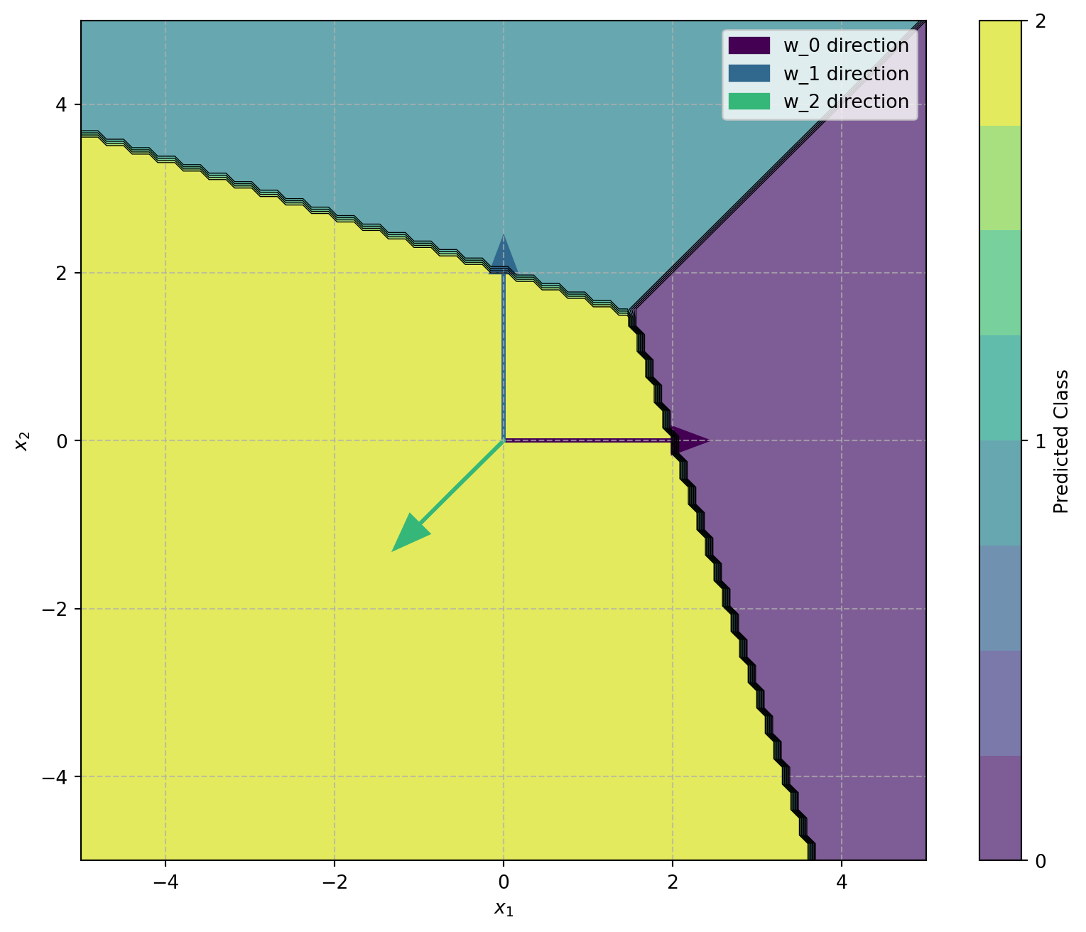
This formulation creates \(K\) decision boundaries, each defined by the hyperplane where \(s_i(x) = s_j(x)\) for classes \(i\) and \(j\).
Figure 1: Multi-class decision boundaries with weight vectors in 2D feature space. Each region represents the area where one class has the highest probability. The arrows indicate the direction of each class’s weight vector.
The geometry of the softmax classifier reveals how it partitions the feature space into regions corresponding to each class. The weight vectors point in the directions that maximize each class’s score, with decision boundaries occurring where adjacent classes have equal scores.
3.1.1 Numerical Stability Considerations
Warning
The softmax function can encounter numerical instability due to the exponential operation. When input values have large magnitudes, exponentials can overflow floating-point representation limits.
The standard numerical stabilization technique subtracts the maximum score from all scores before exponentiation:
This technique is critical for high-dimensional problems like MNIST, where the linear combination of 784 features can produce scores with large magnitudes.
3.2 Cross-Entropy Loss and Gradient
For multi-class classification, the cross-entropy loss measures the divergence between the predicted probability distribution and the one-hot target distribution:
\[
\nabla_{W_k} L = \frac{1}{N}\sum_{i=1}^{N} (a_k^{(i)} - y_k^{(i)})x^{(i)}
\]
This gradient expression is used directly in the optimization algorithms to update the weight vectors.
3.2.1 Optimization Landscape and Gradient Descent
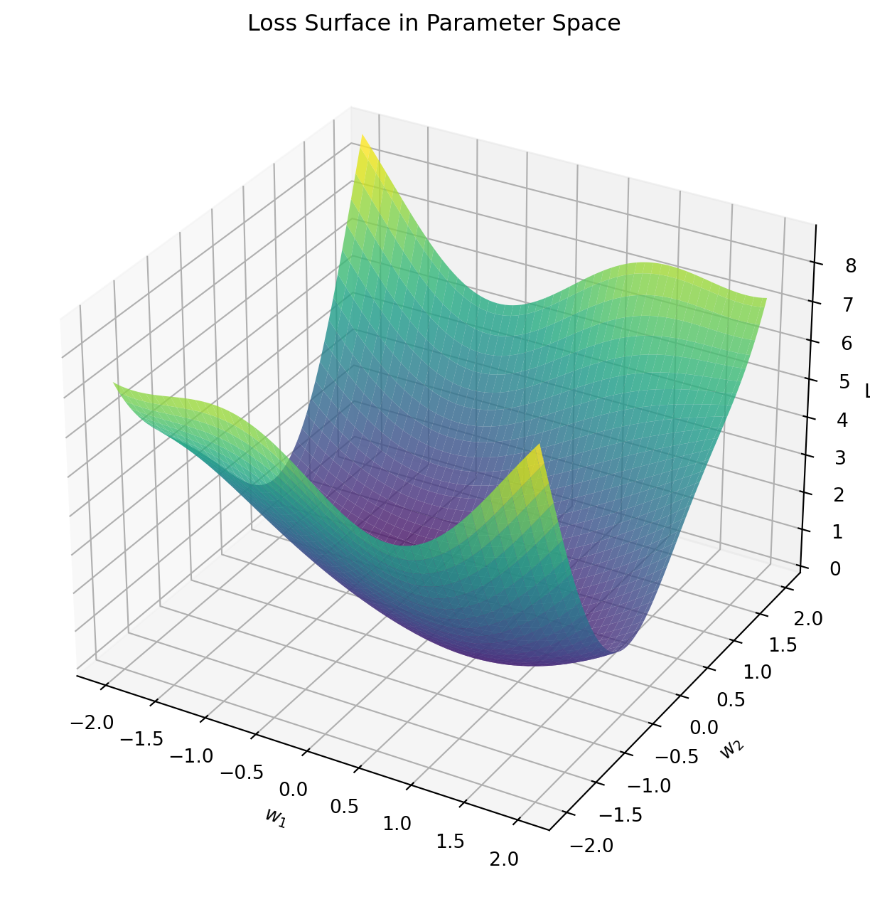
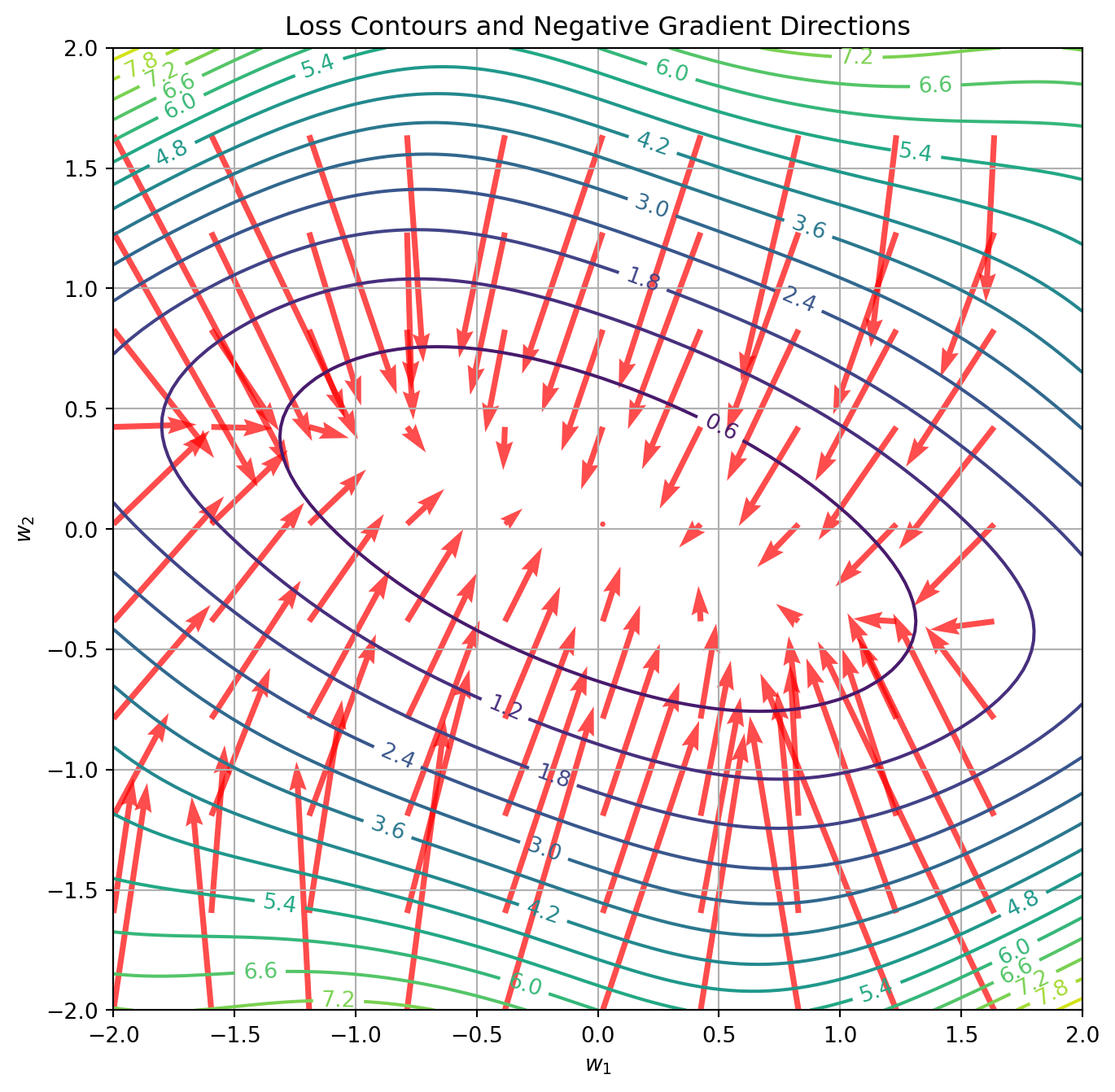
The loss function \(L(w)\) creates a high-dimensional surface in the parameter space. For multi-class logistic regression with \(K\) classes and \(d\) features, this space has \(K \times d\) dimensions plus \(K\) bias terms.
(a) Synthetic 2D visualization of a smooth loss surface with a global minimum and its gradient directions.
(b)
Figure 2
The negative gradient vectors (shown in red) always point in the direction of steepest descent on the loss surface. Gradient descent optimization follows these vectors to approach the global minimum.
3.3 Batch vs. Stochastic Gradient Descent Trajectories
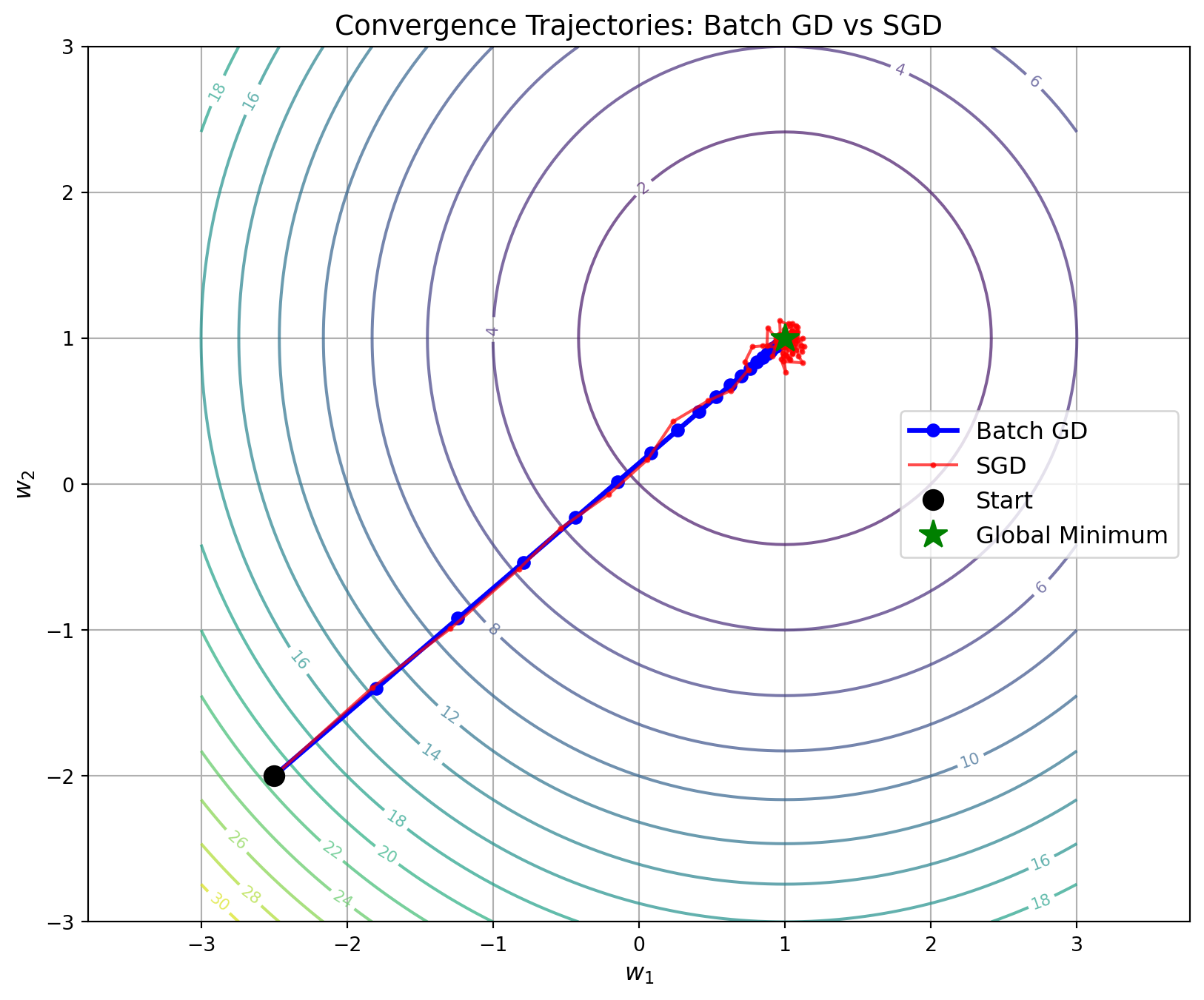
Batch Gradient Descent (BGD) and Stochastic Gradient Descent (SGD) exhibit fundamentally different convergence behaviors due to the nature of their gradient computations.
Figure 3: Simulated convergence paths for Batch Gradient Descent (BGD) and Stochastic Gradient Descent (SGD). BGD follows a straight, smooth path while SGD fluctuates due to gradient noise.
Key differences between optimization methods:
Gradient Estimation:
BGD: Computes the exact gradient over the entire dataset
SGD: Estimates the gradient using a single sample or mini-batch
Convergence Characteristics:
BGD: Smooth, deterministic path
SGD: Noisy, stochastic path that may overshoot but can escape poor local minima
Computational Efficiency:
BGD: \(O(N)\) per update
SGD: \(O(1)\) per update (pure) or \(O(B)\) for mini-batch
3.3.1 Mini-Batch SGD and Computational Considerations
Mini-batch SGD represents a compromise between batch and stochastic methods. Key computational properties:
where \(\sigma^2\) is the variance of the per-sample gradients.
This explains why larger mini-batches allow for more stable convergence and often support larger learning rates.
3.3.2 Computational Complexity and Memory Requirements
The different optimization approaches have distinct computational profiles:
Method
Time Complexity
Memory Requirements
Total Computation to ε-Accuracy
BGD
\(\mathcal{O}(NKD)\) per iteration
\(\mathcal{O}(ND + KD)\)
\(\mathcal{O}(NKD/\varepsilon)\)
Mini-batch SGD
\(\mathcal{O}(BKD)\) per iteration
\(\mathcal{O}(BD + KD)\)
\(\mathcal{O}(KD/\varepsilon^2)\)
Pure SGD
\(\mathcal{O}(KD)\) per iteration
\(\mathcal{O}(D + KD)\)
\(\mathcal{O}(KD/\varepsilon^2)\)
Where: - \(N\) is the dataset size - \(K\) is the number of classes - \(D\) is the input dimensionality - \(B\) is the mini-batch size - \(\varepsilon\) is the target accuracy
For MNIST with \(N=60,000\), \(D=784\), and \(K=10\), these differences are substantial:
The efficiency advantage of stochastic methods typically increases with dataset size, making them particularly valuable for large datasets like MNIST.
3.3.3 Mini-Batch Selection and Optimization
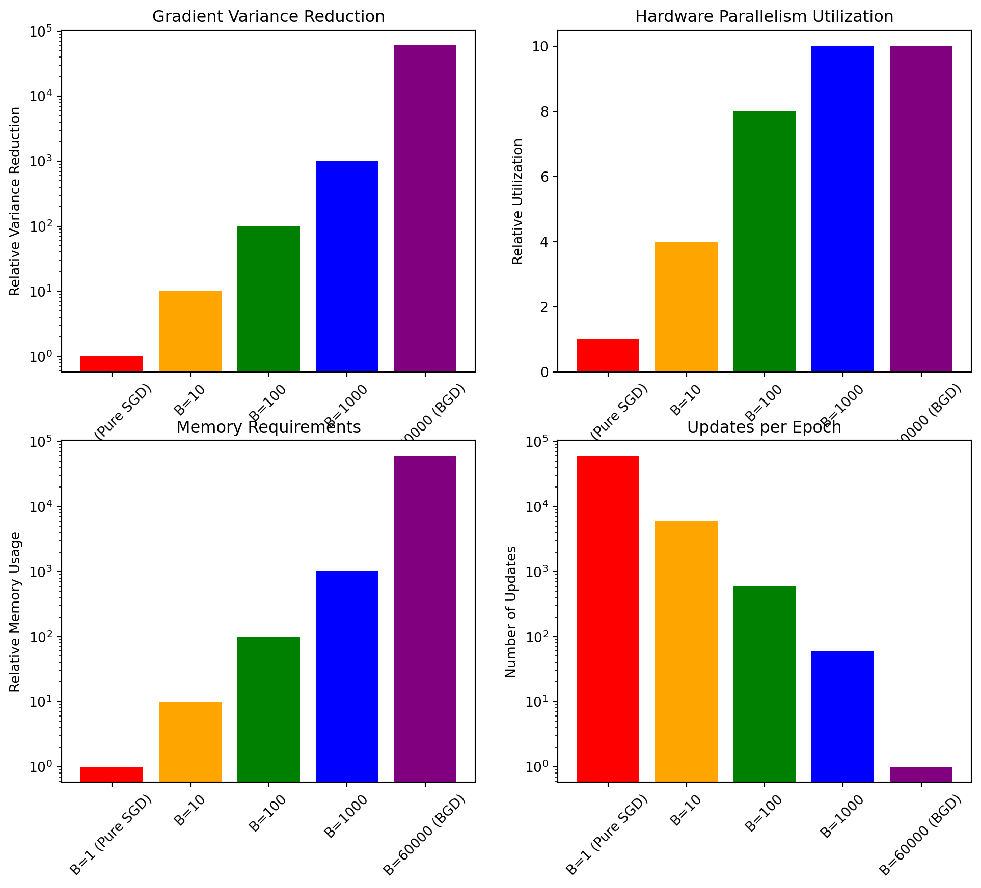
Selecting the appropriate mini-batch size involves a balance between computational efficiency and statistical accuracy:
The tradeoffs between different batch sizes can be summarized in the following table:
Batch Size
Gradient Variance
Hardware Utilization
Memory Requirements
Updates per Epoch
Appropriate Use Cases
B=1 (Pure SGD)
Highest
Lowest
Minimal
Maximum (60,000)
Online learning, memory constraints
B=10
High
Low
Very low
6,000
Quick exploration, limited hardware
B=100
Medium
Good
Moderate
600
Balanced approach for most cases
B=1000
Low
Excellent
High
60
GPU optimization, stable gradients
B=60000 (BGD)
Lowest
Excellent
Highest
1
Convex problems, exact gradients
When selecting a mini-batch size for MNIST, several factors come into play:
Statistical Efficiency: Larger batches provide more accurate gradient estimates with lower variance. The variance of the gradient estimate decreases as \(\mathcal{O}(1/B)\) with batch size \(B\).
Computational Efficiency: Larger batches enable better hardware utilization through parallelization, particularly on GPUs or specialized accelerators.
Memory Requirements: Batch size directly impacts memory usage, with larger batches requiring proportionally more memory.
Update Frequency: Smaller batches allow for more frequent parameter updates per epoch, which can accelerate early learning.
Typical recommendations for MNIST:
Pure SGD (B=1): Provides maximum update frequency but high variance and poor hardware utilization
Small mini-batches (B=10-32): Good for initial exploration or limited hardware
Medium mini-batches (B=64-256): Balanced approach with good hardware utilization
Large mini-batches (B=500+): Better for later stages of training or when using specialized hardware
3.3.4 Comparative Efficiency of Optimization Methods
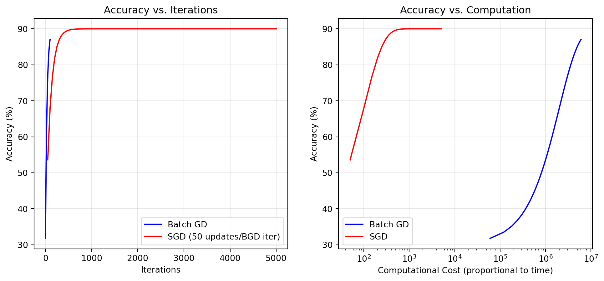
The theoretical and practical efficiency of different optimization methods can be quantified:
For proper comparison between methods, it’s crucial to consider both algorithmic and computational efficiency. While SGD may require more iterations to reach the same accuracy as BGD, each iteration requires significantly less computation. The figure illustrates this fundamental trade-off.
The comparative advantages become more pronounced with increasing dataset size:
Theoretical Convergence Rates:
For strongly convex functions, BGD achieves \(\mathcal{O}(1/t)\) convergence rate
BGD: One parameter update requires \(\mathcal{O}(ND)\) operations
SGD: One parameter update requires \(\mathcal{O}(D)\) operations
Real-world Implications:
For large datasets, SGD often reaches acceptable accuracy with orders of magnitude less computation
BGD’s deterministic trajectory may converge to slightly better final solutions
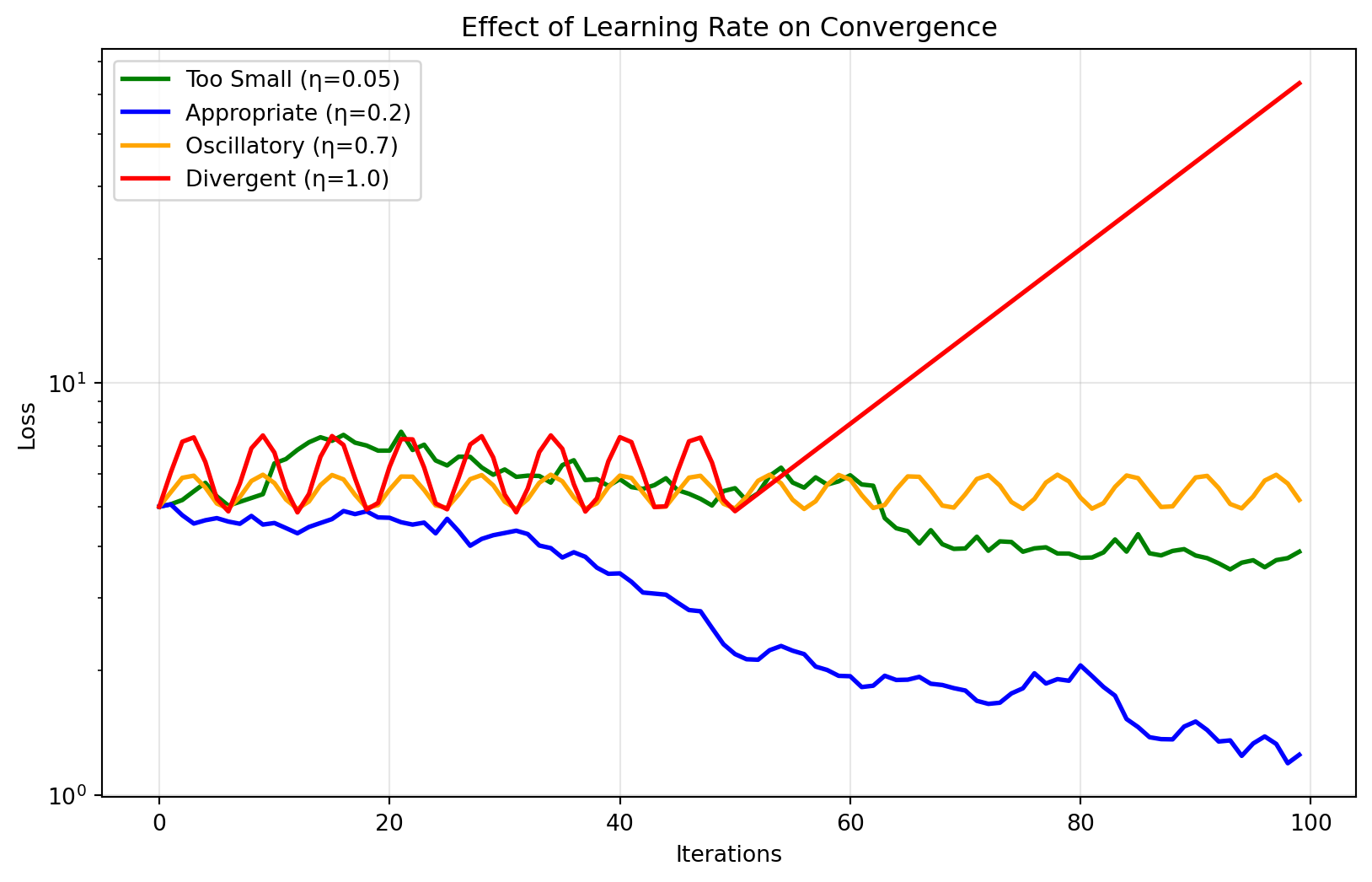
3.4 Learning Rate Dynamics
The learning rate determines the size of parameter updates and dramatically affects convergence behavior:
Learning rate selection involves several critical considerations:
Too small: Convergence is unnecessarily slow, potentially requiring excessive iterations.
Too large: Causes oscillatory behavior or divergence when updates overshoot the minimum.
Optimal range: Typically scales with dataset characteristics and model architecture.
The Polyak-Ruppert averaging theorem suggests the optimal learning rate for SGD scales as \(\eta \propto \frac{1}{\sqrt{t}}\) where \(t\) is the iteration number. This theoretical result motivates common decay schedules:
\[\eta_t = \frac{\eta_0}{\sqrt{1 + \alpha t}}\]
where \(\eta_0\) is the initial rate and \(\alpha\) controls decay speed.
For MNIST with softmax classification, appropriate learning rates typically fall within: - Batch GD: 0.1 - 1.0 - Mini-batch SGD (batch size 100): 0.01 - 0.2 - Pure SGD (batch size 1): 0.001 - 0.05
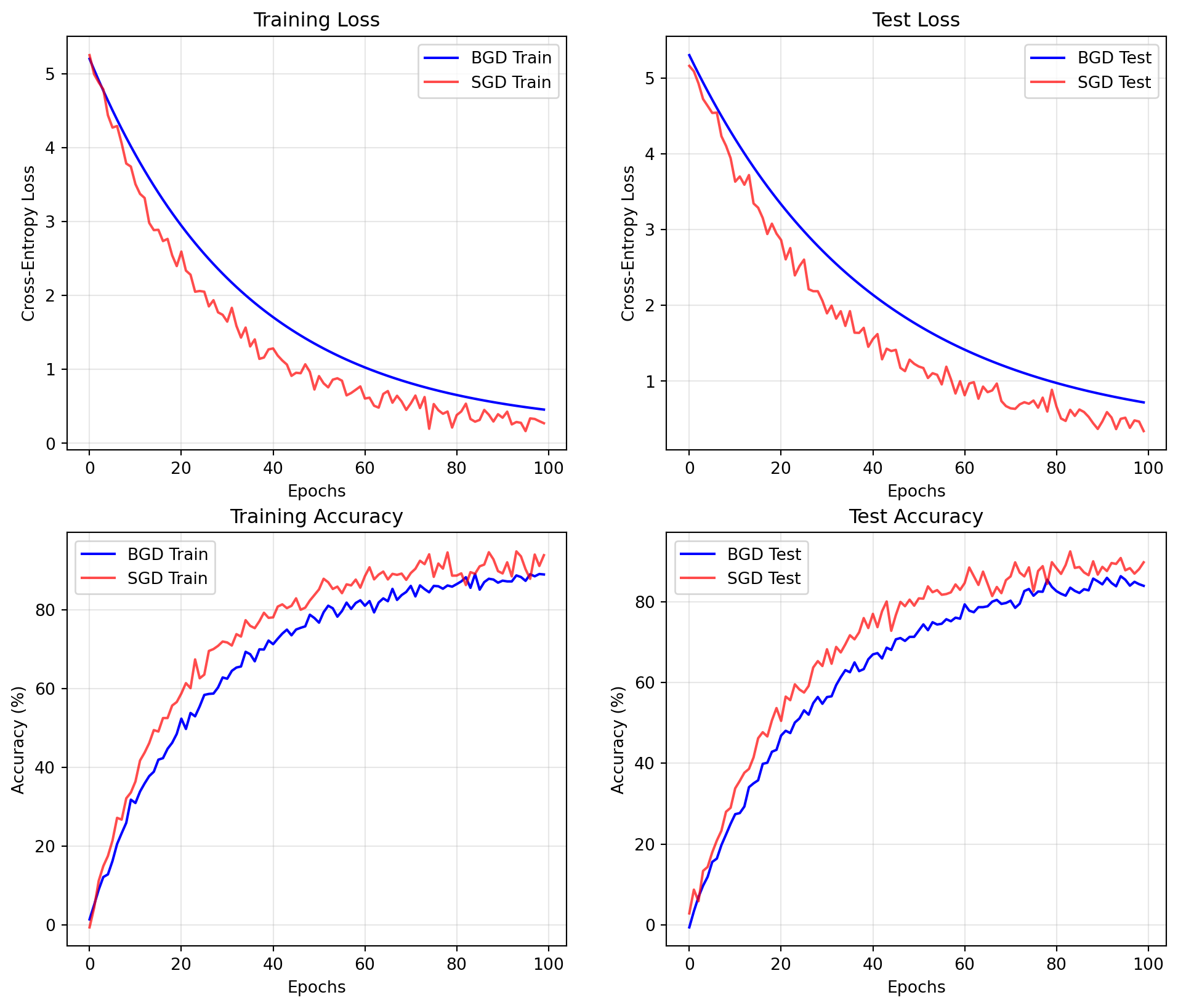
3.4.1 Convergence Analysis
Evaluating optimization performance requires tracking multiple metrics throughout training:
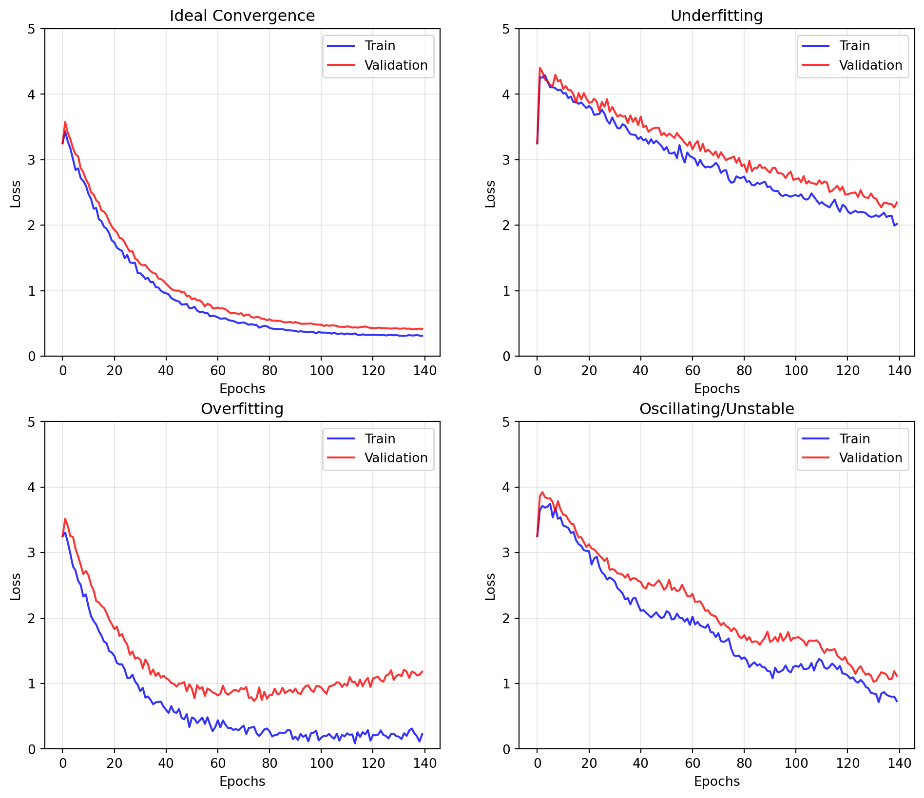
For MNIST with softmax regression, the convergence dynamics typically exhibit:
Training vs. Test Gap: The difference between training and test performance provides insight into generalization. For softmax regression on MNIST, this gap is often small due to the model’s limited capacity.
Epoch-to-Sample Conversion: Comparing batch and stochastic methods requires careful attention to units. One epoch of BGD corresponds to N/B updates in mini-batch SGD, where N is the dataset size and B is the batch size.
Convergence Rate Analysis: Theoretically, SGD and BGD exhibit different convergence rates:
BGD: \(\mathcal{O}(1/t)\) convergence rate with appropriate learning rate
SGD: \(\mathcal{O}(1/\sqrt{t})\) convergence rate, slower in theory but more updates per epoch
Computational Efficiency Metric: A comprehensive comparison incorporates both the convergence rate and computational cost:
For MNIST with 60,000 training samples, BGD requires 60,000 times more computation per update than pure SGD. This often makes SGD more efficient despite its noisier trajectory.
3.4.2 Convergence Theorems and Guarantees
The theoretical foundations of optimization methods provide insights into their behavior:
Convexity and Convergence: For convex functions (like softmax regression), gradient descent with appropriate learning rate is guaranteed to converge to the global minimum.
SGD Convergence Theorem: For strongly convex functions, SGD with decreasing learning rate \(\eta_t = \frac{\eta_0}{1+\lambda t}\) converges in expectation to the optimal solution:
\[\mathbb{E}[\|w_t - w^*\|^2] \leq \frac{C}{t}\]
where \(C\) is a constant depending on the initial distance and gradient variance.
Mini-batch Effect: Theoretically, using a mini-batch of size \(B\) reduces the gradient variance by a factor of \(\frac{1}{B}\), which can allow for proportionally larger learning rates.
These theoretical guarantees provide confidence in the convergence of the optimization methods used for softmax classification on MNIST.
3.5 Weight Visualization and Model Interpretation
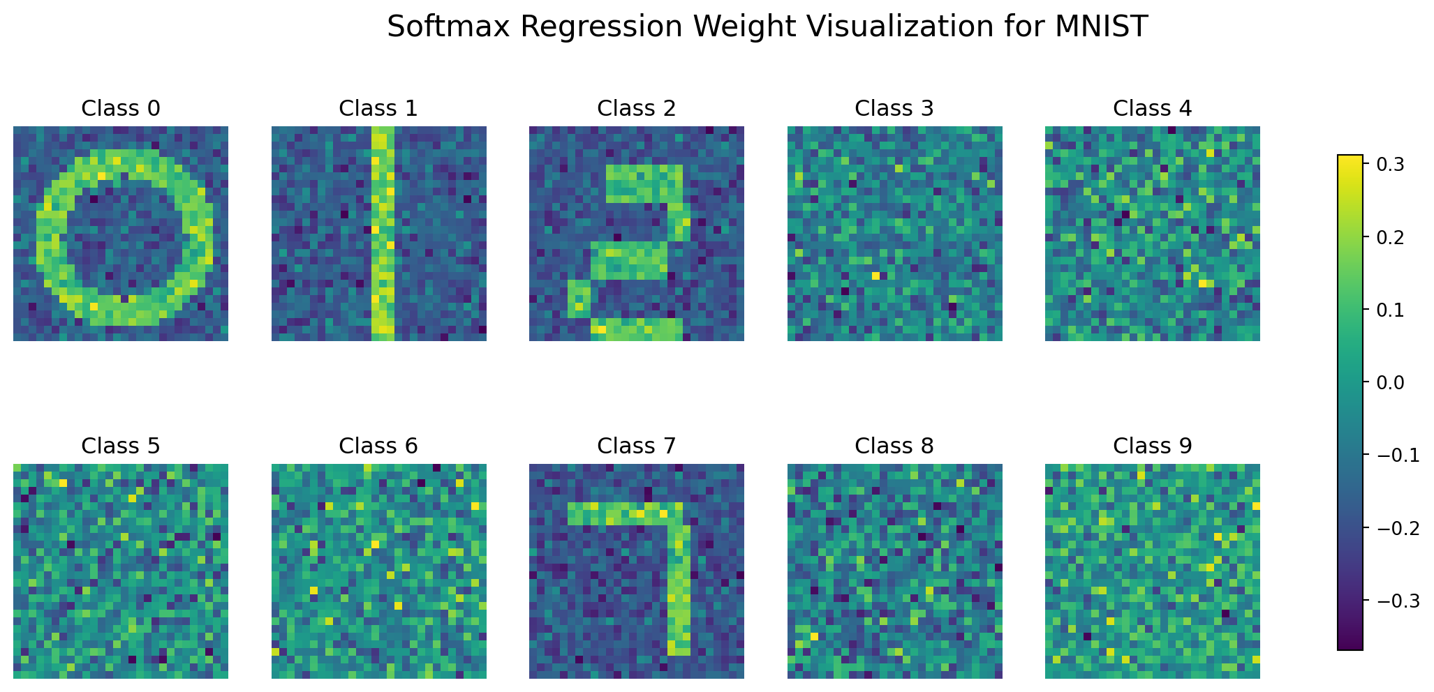
Visualizing the learned weights provides insight into the features the model has identified for each class:
The weight visualization reveals that:
Each weight vector forms a template-like representation of the corresponding digit
Positive weights (warmer colors) indicate features that increase the score for that class
Negative weights (cooler colors) represent features that decrease the score
The templates highlight the discriminative features rather than reconstructing the digits
This visualization demonstrates that multi-class logistic regression learns a set of linear filters, each optimized to detect one class against all others.
3.6 Practical Implementation
For effective implementation of softmax regression on MNIST, consider the following practical strategies:
Normalization: Scale pixel values to the [0,1] range by dividing by 255.
Weight Initialization: Initialize weights with small random values to break symmetry:
W = np.random.randn(n_classes, n_features) *0.01b = np.zeros(n_classes)
Learning Rate Schedule: Implement a decaying learning rate to balance initial progress and final convergence:
Early Stopping: Monitor validation performance to prevent overfitting and unnecessary computation.
These strategies help achieve efficient and effective training while avoiding common pitfalls.
3.6.1 Model Persistence and Evaluation
Proper model persistence enables later analysis and reuse:
# Example format for model persistencemodel_data = {'W': W, # Weight matrix (10 × 784)'b': b, # Bias vector (10,)'n_features': 784, # Number of input features'n_classes': 10, # Number of output classes'hyperparameters': { # Training configuration'learning_rate': learning_rate,'batch_size': batch_size,'n_iterations': n_iterations },'performance': { # Evaluation metrics'train_accuracy': train_accuracy,'test_accuracy': test_accuracy,'train_loss': train_loss,'test_loss': test_loss }}
The HDF5 format specified in the assignment provides an efficient container for these model parameters, preserving numerical precision and array structures.
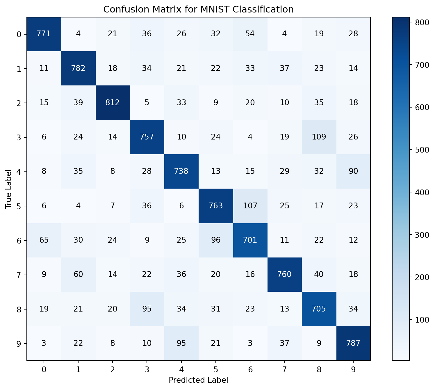
For comprehensive evaluation, compute the confusion matrix:
The confusion matrix reveals systematic patterns in model errors, providing insight into similar digit pairs that the model struggles to differentiate. This information can guide potential model improvements or feature engineering efforts.
Source Code
---title: "Homework #6 -- Getting Started Guide"#subtitle: "EE 541: Computational Deep Learning"#author: "Spring 2025"format: html: toc: true toc-depth: 3 number-sections: true code-fold: true code-tools: true code-link: true theme: cosmo #include-before-body: # - file: ../../macros.mdjupyter: python3execute: echo: true warning: false---{{< include hw06-q01.qmd >}}{{< include hw06-q02.qmd >}}{{< include hw06-q03.qmd >}}