Homework #8 – Getting Started Guide

0 PyTorch for Deep Learning

0.1 What is PyTorch?

PyTorch is an open-source machine learning framework developed by Facebook’s AI Research lab (FAIR). It evolved from Torch, a scientific computing framework built in Lua. PyTorch reimplemented Torch’s core functionality in Python while adding automatic differentiation capabilities.

The fundamental distinction between PyTorch and frameworks like early TensorFlow lies in their computational graph approach. PyTorch uses a dynamic computational graph (“define-by-run”), where the graph is constructed on-the-fly during execution. This offers greater flexibility for debugging and developing complex models.

PyTorch uses a hybrid architecture: the frontend is Python for ease of use and rapid development, while the computational backend is implemented in C++ and CUDA for performance. This architecture provides:

  • Python’s flexibility and ecosystem integration
  • C++’s execution speed for computation-intensive operations
  • CUDA’s parallel computing capabilities for GPU acceleration

The design focuses on:

  • Tensor computation with strong GPU acceleration
  • Automatic differentiation for building and training neural networks
  • Deep neural network APIs built on a tape-based autograd system

This hybrid approach resolves the apparent paradox of implementing computationally intensive tasks in Python. While Python itself is relatively slow, the actual numeric computations in PyTorch are performed by optimized C++/CUDA code with minimal Python overhead.

0.2 GPU Acceleration

Modern deep learning relies heavily on GPU computing to accelerate matrix operations. PyTorch provides built-in support for NVIDIA GPUs through CUDA and for Apple Silicon hardware through Metal Performance Shaders (MPS).

# Check if GPU is available and set device accordingly
device = torch.device("cuda:0" if torch.cuda.is_available() else "cpu")

# For Mac users with Apple Silicon
if not torch.cuda.is_available():
    device = torch.device("mps" if torch.backends.mps.is_available() else "cpu")

print(f"Using device: {device}")
Note

GPU acceleration typically provides speed improvements of 10-100x compared to CPU-only training for large neural networks. This speedup comes from parallelizing specific operations:

  • Matrix multiplications in linear layers see massive parallelization benefits
  • Convolutional operations are highly optimized for GPU execution
  • Batch processing allows parallel handling of multiple samples

Not all operations benefit equally: recurrent neural networks (RNNs) have sequential dependencies that limit parallelization, and reinforcement learning algorithms with sequential decision processes may see less dramatic speedups. Modern architectures like Transformers were specifically designed to maximize GPU parallelization potential.

To use GPU acceleration effectively:

  • Move the model to the GPU

    model = model.to(device)
  • Move input data to the GPU before forward passes

    inputs, labels = inputs.to(device), labels.to(device)
  • Retrieve CPU tensors when needed (e.g., for numpy operations or visualization)

    cpu_tensor = gpu_tensor.cpu()

Performance considerations when using GPUs:

  • Data transfer overhead: Moving data between CPU and GPU is relatively slow
  • Batch size: Larger batch sizes utilize GPU parallelism better, but may cause memory issues
  • Mixed precision: Using half-precision (FP16) can significantly accelerate training on modern GPUs
  • Memory management: Large models or datasets may require techniques like gradient checkpointing or model parallelism

0.3 Tensors: PyTorch’s Core Data Structure

0.3.1 Tensor Basics

Tensors are multi-dimensional arrays similar to NumPy’s ndarray, but with added GPU support and automatic differentiation capabilities:

# Create a tensor directly
x = torch.tensor([[1, 2], [3, 4]], dtype=torch.float32)

# Create a tensor from NumPy array
import numpy as np
np_array = np.array([[1, 2], [3, 4]])
x = torch.from_numpy(np_array)

# Create special tensors
zeros = torch.zeros(2, 3)               # Tensor of zeros
ones = torch.ones(2, 3)                 # Tensor of ones
rand = torch.rand(2, 3)                 # Random uniform [0, 1)
randn = torch.randn(2, 3)               # Random normal (mean=0, var=1)

0.3.2 Tensor Operations

PyTorch provides extensive operations for tensor manipulation:

# Basic arithmetic
a = torch.tensor([1, 2, 3])
b = torch.tensor([4, 5, 6])
c = a + b                         # Element-wise addition
d = a * b                         # Element-wise multiplication
e = torch.matmul(a, b)            # Dot product

# Reshaping
f = torch.randn(4, 4)
g = f.view(16)                    # Reshape to 1D tensor
h = f.view(-1, 8)                 # -1 dimension is inferred

0.3.3 Automatic Differentiation

The key feature distinguishing tensors from NumPy arrays is automatic differentiation through the autograd system:

x = torch.tensor([2.0], requires_grad=True)
y = x**2 + 3*x + 1
y.backward()                      # Compute gradient dy/dx
print(x.grad)                     # dy/dx = 2x + 3 = 7 at x=2

This system enables the efficient computation of gradients for optimizing neural networks.

0.4 Dataset Handling in PyTorch

PyTorch provides a standardized way to work with datasets through the Dataset and DataLoader classes.

0.4.1 Built-in Datasets

PyTorch’s torchvision module includes many popular computer vision datasets:

import torchvision
import torchvision.transforms as transforms

# Define transformations
transform = transforms.Compose([
    transforms.ToTensor(),  # Convert images to tensors
    transforms.Normalize((0.5,), (0.5,))  # Normalize with mean and std
])

# Load MNIST dataset
train_dataset = torchvision.datasets.MNIST(
    root='./data',
    train=True,
    download=True,
    transform=transform
)

# Create a DataLoader
train_loader = torch.utils.data.DataLoader(
    train_dataset,
    batch_size=64,
    shuffle=True
)

The transforms module allows for data preprocessing and augmentation:

# More complex transformation pipeline
transform = transforms.Compose([
    transforms.RandomHorizontalFlip(),  # Randomly flip images horizontally
    transforms.RandomRotation(10),      # Randomly rotate up to 10 degrees
    transforms.ToTensor(),
    transforms.Normalize((0.5,), (0.5,))
])

0.4.2 DataLoader Features

The DataLoader class provides several important features:

dataloader = torch.utils.data.DataLoader(
    dataset,
    batch_size=32,        # Number of samples per batch
    shuffle=True,         # Shuffle the data
    num_workers=4,        # Parallel data loading threads
    pin_memory=True       # Better performance with CUDA
)
  • Batching: Groups samples into batches for efficient processing
  • Shuffling: Randomizes the order of samples in each epoch
  • Parallelism: Loads data using multiple worker processes
  • Memory pinning: Optimizes memory transfers to CUDA devices

0.5 Building Neural Networks

0.5.1 Understanding nn.Module

The foundation of neural network models in PyTorch is the nn.Module class. All network architectures inherit from this base class:

import torch.nn as nn

class SimpleNN(nn.Module):
    def __init__(self, input_size, hidden_size, output_size):
        super(SimpleNN, self).__init__()
        self.flatten = nn.Flatten()
        self.fc1 = nn.Linear(input_size, hidden_size)
        self.relu = nn.ReLU()
        self.fc2 = nn.Linear(hidden_size, output_size)
    
    def forward(self, x):
        x = self.flatten(x)
        x = self.fc1(x)
        x = self.relu(x)
        x = self.fc2(x)
        return x

Key aspects of nn.Module:

  • Initialization: The __init__ method defines the layers and components
  • Forward pass: The forward method defines how data flows through the layers
  • Parameter tracking: All parameters (weights and biases) are automatically tracked
  • Module nesting: Modules can contain other modules for hierarchical designs

0.5.2 nn.Sequential vs Custom nn.Module

nn.Sequential provides a container for a linear sequence of layers:

model = nn.Sequential(
    nn.Flatten(),
    nn.Linear(784, 128),
    nn.ReLU(),
    nn.Linear(128, 10)
)

While nn.Sequential is concise, custom nn.Module subclasses offer several advantages:

  • Complex data flow: Support for skip connections, multiple inputs/outputs, etc.
  • Conditional computation: Dynamic behavior based on input or state
  • Reusable components: Define custom building blocks that can be reused
  • Programmatic creation: Create layers based on parameters or loops

Example of programmatic layer creation with nn.Module:

class MLP(nn.Module):
    def __init__(self, input_size, hidden_sizes, output_size):
        super(MLP, self).__init__()
        
        # Create layers programmatically
        self.layers = nn.ModuleList()
        all_sizes = [input_size] + hidden_sizes + [output_size]
        
        for i in range(len(all_sizes) - 1):
            self.layers.append(nn.Linear(all_sizes[i], all_sizes[i+1]))
            if i < len(all_sizes) - 2:  # No activation after the last layer
                self.layers.append(nn.ReLU())
    
    def forward(self, x):
        x = x.view(x.size(0), -1)  # Flatten
        for layer in self.layers:
            x = layer(x)
        return x

0.5.3 Layer Types

PyTorch provides various layer types for neural network construction:

# Linear (fully connected) layer
linear = nn.Linear(in_features, out_features, bias=True)

# Common activation functions
relu = nn.ReLU()
leaky_relu = nn.LeakyReLU(negative_slope=0.01)
sigmoid = nn.Sigmoid()
tanh = nn.Tanh()

# Batch normalization
batch_norm = nn.BatchNorm1d(num_features)

0.6 Parameters and Training

0.6.1 Loss Functions

Loss functions measure the error between predictions and ground truth. PyTorch provides many common loss functions:

# Binary classification
bce_loss = nn.BCELoss()                        # Binary Cross Entropy (requires sigmoid activation)
bce_with_logits = nn.BCEWithLogitsLoss()       # Combines sigmoid + BCELoss

# Multi-class classification
ce_loss = nn.CrossEntropyLoss()                # Combines LogSoftmax + NLLLoss
nll_loss = nn.NLLLoss()                        # Negative Log Likelihood (requires log-softmax activations)

# Regression
mse_loss = nn.MSELoss()                        # Mean Squared Error
l1_loss = nn.L1Loss()                          # Mean Absolute Error
smooth_l1 = nn.SmoothL1Loss()                  # Huber loss
Note

CrossEntropyLoss and BCEWithLogitsLoss combine an activation function with the loss calculation. When using these, do not apply softmax or sigmoid to your model’s output:

# With CrossEntropyLoss (correct)
outputs = model(inputs)  # Raw logits
loss = criterion(outputs, labels)

# NOT recommended
outputs = model(inputs)  # Raw logits
outputs = F.softmax(outputs, dim=1)  # Unnecessary softmax
loss = criterion(outputs, labels)    # This will produce incorrect results

The integrated approach improves numerical stability by avoiding operations like exp(x) for large x values.

0.6.2 Optimizers

Optimizers update model parameters based on gradients. The two most widely used in practice are:

# SGD (Stochastic Gradient Descent)
optimizer = optim.SGD(model.parameters(), lr=0.01, momentum=0.9)

# Adam (Adaptive Moment Estimation)
optimizer = optim.Adam(model.parameters(), lr=0.001, betas=(0.9, 0.999))

Optimizer selection guidelines: - SGD: Often preferred for simpler models or when generalization is crucial - Adam: Faster convergence for deep networks and complex tasks

Other optimizers have specific use cases: - RMSprop: Effective for recurrent neural networks - AdamW: Improved weight decay implementation compared to Adam - LBFGS: Second-order optimization method, useful for smaller datasets

0.6.3 Weight Initialization

Proper weight initialization is crucial for neural network training. PyTorch provides initialization functions in the nn.init module:

def init_weights(m):
    if isinstance(m, nn.Linear):
        # Kaiming/He initialization (good for ReLU)
        nn.init.kaiming_normal_(m.weight, mode='fan_in', nonlinearity='relu')
        if m.bias is not None:
            nn.init.constant_(m.bias, 0)

# Apply to all layers
model.apply(init_weights)

Common initialization methods: - Xavier/Glorot: Suitable for tanh or sigmoid activations - Kaiming/He: Better for ReLU activations - Orthogonal: Helpful for recurrent networks

Note

PyTorch uses a variant of Kaiming initialization by default for convolutional and linear layers.

The trailing underscore in kaiming_normal_() indicates an in-place operation—a PyTorch convention for functions that modify tensors directly rather than returning new ones. This approach is memory-efficient because it avoids allocating new memory for large tensors, particularly important during initialization of models with millions of parameters.

0.7 Model Training and Evaluation

0.7.1 Training Loop

A complete training loop in PyTorch follows this pattern:

def train_model(model, train_loader, val_loader, criterion, optimizer, num_epochs, device):
    train_losses = []
    val_losses = []
    
    for epoch in range(num_epochs):
        # Training phase
        model.train()
        running_loss = 0.0
        
        for inputs, labels in train_loader:
            inputs, labels = inputs.to(device), labels.to(device)
            
            # Zero the parameter gradients
            optimizer.zero_grad()
            
            # Forward pass
            outputs = model(inputs)
            loss = criterion(outputs, labels)
            
            # Backward pass and optimize
            loss.backward()
            optimizer.step()
            
            running_loss += loss.item()
        
        epoch_train_loss = running_loss / len(train_loader)
        train_losses.append(epoch_train_loss)
        
        # Validation phase
        model.eval()
        running_loss = 0.0
        
        with torch.no_grad():  # Disable gradient computation
            for inputs, labels in val_loader:
                inputs, labels = inputs.to(device), labels.to(device)
                outputs = model(inputs)
                loss = criterion(outputs, labels)
                running_loss += loss.item()
        
        epoch_val_loss = running_loss / len(val_loader)
        val_losses.append(epoch_val_loss)
        
        print(f'Epoch {epoch+1}/{num_epochs} | '
              f'Train Loss: {epoch_train_loss:.4f} | '
              f'Val Loss: {epoch_val_loss:.4f}')
    
    return train_losses, val_losses

Key components of the training loop:

  • Set the model to training mode with model.train()
  • Zero gradients before the forward pass with optimizer.zero_grad()
  • Compute the loss and perform backpropagation with loss.backward()
  • Update parameters with optimizer.step()
  • Set the model to evaluation mode with model.eval() during validation
  • Disable gradient calculation with torch.no_grad() during validation

0.7.2 Learning Rate Scheduling

Learning rate schedulers adjust the learning rate during training:

# Step learning rate scheduler
scheduler = torch.optim.lr_scheduler.StepLR(optimizer, step_size=10, gamma=0.1)

# Reduce learning rate on plateau
scheduler = torch.optim.lr_scheduler.ReduceLROnPlateau(optimizer, mode='min', factor=0.1, patience=5)

# In the training loop
for epoch in range(num_epochs):
    # Train for one epoch
    train(...)
    
    # Update the learning rate
    scheduler.step()  # For StepLR
    # or
    scheduler.step(val_loss)  # For ReduceLROnPlateau

0.7.3 Model Evaluation

To evaluate model performance, calculate metrics like accuracy, precision, recall, or F1-score:

def evaluate_model(model, test_loader, device):
    model.eval()
    correct = 0
    total = 0
    
    with torch.no_grad():
        for inputs, labels in test_loader:
            inputs, labels = inputs.to(device), labels.to(device)
            outputs = model(inputs)
            _, predicted = torch.max(outputs.data, 1)
            total += labels.size(0)
            correct += (predicted == labels).sum().item()
    
    accuracy = 100 * correct / total
    return accuracy

0.8 Visualizing and Analyzing Results

0.8.1 Learning Curves

Learning curves help identify overfitting or underfitting:

import matplotlib.pyplot as plt

def plot_learning_curves(train_losses, val_losses, train_accs=None, val_accs=None):
    epochs = range(1, len(train_losses) + 1)
    
    fig, ax1 = plt.subplots(figsize=(10, 6))
    
    # Plot losses
    color = 'tab:blue'
    ax1.set_xlabel('Epochs')
    ax1.set_ylabel('Loss', color=color)
    ax1.plot(epochs, train_losses, color=color, label='Training Loss')
    ax1.plot(epochs, val_losses, color='tab:orange', label='Validation Loss')
    ax1.tick_params(axis='y', labelcolor=color)
    
    # Plot accuracies if provided
    if train_accs and val_accs:
        ax2 = ax1.twinx()
        color = 'tab:red'
        ax2.set_ylabel('Accuracy (%)', color=color)
        ax2.plot(epochs, train_accs, color=color, linestyle='--', label='Training Acc')
        ax2.plot(epochs, val_accs, color='tab:green', linestyle='--', label='Validation Acc')
        ax2.tick_params(axis='y', labelcolor=color)
    
    fig.tight_layout()
    fig.legend(loc='upper right', bbox_to_anchor=(1,1), bbox_transform=ax1.transAxes)
    plt.title('Training and Validation Metrics')
    plt.show()

0.9 Saving and Loading Models

Saving and loading models in PyTorch is essential for preserving training progress and deploying models.

0.9.1 Basic Model Saving

The simplest way to save a model is to save its state dictionary:

# Save model state dictionary
torch.save(model.state_dict(), 'model.pth')

# Load model state dictionary
model = MyModel()  # Create an instance of the model
model.load_state_dict(torch.load('model.pth'))
model.eval()  # Set to evaluation mode

0.9.2 Comprehensive Checkpointing

For more comprehensive checkpointing that allows resuming training:

def save_checkpoint(model, optimizer, epoch, scheduler, best_accuracy, filepath):
    """Save model checkpoint with all training state."""
    checkpoint = {
        'epoch': epoch,
        'model_state_dict': model.state_dict(),
        'optimizer_state_dict': optimizer.state_dict(),
        'scheduler_state_dict': scheduler.state_dict() if scheduler else None,
        'best_accuracy': best_accuracy
    }
    torch.save(checkpoint, filepath)
    print(f"Checkpoint saved at {filepath}")

def load_checkpoint(model, optimizer, scheduler, filepath):
    """Load model checkpoint with all training state."""
    checkpoint = torch.load(filepath)
    model.load_state_dict(checkpoint['model_state_dict'])
    optimizer.load_state_dict(checkpoint['optimizer_state_dict'])
    if scheduler and 'scheduler_state_dict' in checkpoint:
        scheduler.load_state_dict(checkpoint['scheduler_state_dict'])
    epoch = checkpoint['epoch']
    best_accuracy = checkpoint['best_accuracy'] if 'best_accuracy' in checkpoint else 0
    print(f"Checkpoint loaded from {filepath} (epoch {epoch})")
    return epoch, best_accuracy

0.9.3 Including Variables in Filenames

Including timestamp and performance metrics in filenames helps organize checkpoints:

import time
import datetime

def get_checkpoint_filename(model_name, epoch, accuracy=None):
    """Generate a checkpoint filename with timestamp and metrics."""
    timestamp = datetime.datetime.now().strftime("%Y%m%d_%H%M%S")
    if accuracy is not None:
        return f"{model_name}_{timestamp}_epoch{epoch}_acc{accuracy:.2f}.pth"
    else:
        return f"{model_name}_{timestamp}_epoch{epoch}.pth"

# Usage in training loop
for epoch in range(start_epoch, num_epochs):
    # Training code...
    
    # Save checkpoint periodically
    if (epoch + 1) % 10 == 0:
        filepath = get_checkpoint_filename("resnet18", epoch, val_accuracy)
        save_checkpoint(model, optimizer, epoch, scheduler, best_accuracy, filepath)

This approach organizes checkpoints with relevant information for easy identification.

0.9.4 TorchScript for Deployment

TorchScript is a way to serialize and optimize PyTorch models for production deployment:

# Convert to TorchScript using tracing
example_input = torch.rand(1, 3, 224, 224)
traced_model = torch.jit.trace(model, example_input)
traced_model.save("model_traced.pt")

# Or using scripting (preferred for models with control flow)
scripted_model = torch.jit.script(model)
scripted_model.save("model_scripted.pt")

print("Model saved for deployment")

# Loading a TorchScript model
loaded_model = torch.jit.load("model_scripted.pt")

TorchScript offers several advantages for deployment:

  1. Language independence: Run in C++ environments without Python
  2. Optimization: Optimize the model for inference performance
  3. Portability: Deploy to various platforms, including mobile devices
  4. Graph-level optimizations: Fuse operations for better performance

TorchScript models can be:

  • Used in production environments where Python is not available
  • Integrated into larger applications written in C++
  • Deployed on resource-constrained devices
  • Run with optimized inference performance

0.10 Inside PyTorch: Exploring the Source Code

Understanding PyTorch’s internal implementation provides deeper insights into how it achieves both high performance and flexibility.

0.10.1 Finding Source Code

For installed packages, find the source directory with:

import torch
import torch.nn as nn
import inspect

# Find the source file of a class
print(inspect.getsourcefile(nn.Linear))

0.10.2 Linear Layer Implementation

Let’s examine the key components of the nn.Linear implementation:

# Simplified version of nn.Linear's core functionality
def linear_forward(input, weight, bias=None):
    output = input.matmul(weight.t())
    if bias is not None:
        output += bias
    return output

The actual PyTorch implementation includes additional optimizations and special cases, but the core operation is a simple matrix multiplication followed by a bias addition. However, this Python-like code ultimately calls optimized C++/CUDA implementations that perform the actual computation.

0.10.3 Loss Function Implementation

The CrossEntropyLoss combines log softmax and negative log-likelihood:

# Simplified version of CrossEntropyLoss's core functionality
def cross_entropy_loss(input, target, weight=None, reduction='mean'):
    log_softmax = F.log_softmax(input, 1)
    loss = F.nll_loss(log_softmax, target, weight=weight, reduction=reduction)
    return loss

The combined implementation avoids numerical instability issues that could arise from separate softmax and log operations. For large values, direct computation of softmax can lead to overflow, while the combined approach uses log-sum-exp tricks to maintain numerical stability.

0.10.4 Autograd Implementation

The automatic differentiation system is built around the concept of a computational graph:

  • Forward Pass: Tensors flow through operations, recording the computation history
  • Backward Pass: Gradients are computed by applying the chain rule, flowing backward through the graph

Each operation in PyTorch implements both a forward function and a backward function that defines how gradients propagate. The C++ backend implements these operations efficiently while the Python frontend provides the user interface.

0.11 PyTorch Conventions and Patterns

PyTorch follows several conventions that are helpful to understand:

0.11.1 Naming Conventions

  • In-place operations: Functions ending with an underscore (tensor.add_()) modify the tensor in place. This approach is memory-efficient because it avoids allocating new memory for large tensors, particularly important during initialization of models with millions of parameters.
  • Parameter classes: Classes starting with Parameter represent learnable parameters
  • Module hooks: Functions with hook in the name are used for intercepting forward/backward passes

0.11.2 Tensor Dimension Ordering

PyTorch typically follows this dimension ordering convention:

  • Batch dimension first (N)
  • For images: [N, C, H, W] (batch, channels, height, width)
  • For sequences: [N, L, F] (batch, sequence length, features)

0.11.3 The .detach() Method

The detach() method disconnects a tensor from the computation graph:

# Create a tensor requiring gradients
x = torch.tensor([1.0, 2.0, 3.0], requires_grad=True)
y = x * 2

# Detach y from the computation graph
z = y.detach()

# z's operations won't affect x's gradients
z = z * 3
z.sum().backward()  # This won't affect x.grad

This is useful when you want to use a tensor’s values without tracking its computational history. Common use cases include:

  • Preventing gradient flow through certain parts of a network
  • Using intermediate results for visualization or logging without affecting gradients
  • Converting tensors to NumPy arrays for interoperability with other libraries
  • Implementing algorithms that require stopping gradient propagation, like GANs or certain reinforcement learning techniques

1 MNIST Logistic Classification with PyTorch

The MNIST dataset is a collection of 28×28 grayscale images of handwritten digits (0-9), consisting of 60,000 training examples and 10,000 test examples. For this problem, you’ll implement a logistic classifier using PyTorch’s neural network modules.

1.1 Custom Dataset for HDF5 Files

The MNIST data for this assignment is stored in HDF5 (.hdf5) format, which is commonly used for scientific datasets. HDF5 files can store structured data and support efficient reading of subsets of data. To work with these files in PyTorch, a custom dataset class is needed.

In PyTorch, datasets are accessed through the Dataset class, which requires implementing:

  • __init__: Initialize the dataset, open files, prepare data
  • __len__: Return the number of samples in the dataset
  • __getitem__: Return a specific sample at a given index
  • __del__: (Optional) Clean up resources when the dataset is no longer used

For HDF5 files specifically, the implementation needs to handle the file connections:

import h5py
import torch
from torch.utils.data import Dataset

class MNISTHDF5Dataset(Dataset):
    def __init__(self, file_path, transform=None):
        """Initialize the dataset by opening the HDF5 file."""
        self.file = h5py.File(file_path, 'r')
        self.images = self.file['images']
        self.labels = self.file['labels']
        self.transform = transform
    
    def __len__(self):
        """Return the number of samples in the dataset."""
        return len(self.images)
    
    def __getitem__(self, idx):
        """Return a specific sample and its label."""
        # Get image and flatten it to match a logistic classifier's input format
        image = torch.FloatTensor(self.images[idx]).view(-1)  # 28x28 -> 784
        label = int(self.labels[idx])
        
        if self.transform:
            image = self.transform(image)
        
        return image, label
    
    def __del__(self):
        """Close the HDF5 file when the dataset is no longer used."""
        if hasattr(self, 'file'):
            self.file.close()
Note

The __del__ method ensures that the HDF5 file is properly closed when the dataset is no longer used. This is important for resource management, especially when working with multiple datasets.

With this dataset, a DataLoader can be created to handle batching and shuffling:

from torch.utils.data import DataLoader

# Create datasets
train_dataset = MNISTHDF5Dataset('mnist_traindata.hdf5')
test_dataset = MNISTHDF5Dataset('mnist_testdata.hdf5')

# Create dataloaders
batch_size = 100  # As specified in the assignment
train_loader = DataLoader(train_dataset, batch_size=batch_size, shuffle=True)
test_loader = DataLoader(test_dataset, batch_size=batch_size, shuffle=False)

1.1.1 Interacting with Datasets and DataLoaders

PyTorch datasets and dataloaders provide convenient ways to access and visualize your data. Here’s how to interact with them:

1.1.1.1 Accessing Individual Samples

You can access individual samples directly from the dataset:

# Get a single sample from the dataset
image, label = train_dataset[0]

print(f"Image shape: {image.shape}")
print(f"Label: {label}")

1.1.1.2 Visualizing Images

To visualize an image from the MNIST dataset:

import matplotlib.pyplot as plt

# Reshape the flattened image back to 28x28
plt.figure(figsize=(3, 3))
plt.imshow(image.reshape(28, 28), cmap='gray')
plt.title(f"Digit: {label}")
plt.axis('off')
plt.show()

1.1.1.3 Working with Batches

DataLoaders provide batches of data as iterables:

# Get a single batch
dataiter = iter(train_loader)
images, labels = next(dataiter)

print(f"Batch shape: {images.shape}")  # Should be [batch_size, 784]
print(f"Labels shape: {labels.shape}")  # Should be [batch_size]

1.1.1.4 Visualizing a Batch of Images

To visualize multiple images from a batch:

# Display a grid of images from a batch
plt.figure(figsize=(12, 6))
for i in range(10):  # Display first 10 images from the batch
    plt.subplot(2, 5, i + 1)
    plt.imshow(images[i].reshape(28, 28), cmap='gray')
    plt.title(f"Digit: {labels[i].item()}")
    plt.axis('off')
plt.tight_layout()
plt.show()

1.1.1.5 Iterating Through the DataLoader

DataLoaders are designed to be used in loops, which is perfect for training neural networks:

# Example of iterating through a DataLoader
num_batches = 0
for images, labels in train_loader:
    num_batches += 1
    # Process the batch here...
    
    # Break after a few batches for demonstration
    if num_batches == 3:
        break

print(f"Total number of batches: {len(train_loader)}")

1.2 Single-Layer Logistic Classifier with nn.Sequential

For a logistic classifier, we need a single fully-connected (linear) layer that maps the input features to class scores. With MNIST images (28×28), the input size is 784 (flattened) and the output size is 10 (for digits 0-9).

The nn.Sequential container provides a simple way to define this model:

import torch.nn as nn

# Define model dimensions using variables
input_size = 28 * 28  # Flattened input image dimensions
num_classes = 10      # Number of output classes (digits 0-9)

# Create the model with a single linear layer
model = nn.Sequential(
    nn.Linear(input_size, num_classes)
)

print(model)
Important

The above model outputs raw class scores (logits), not probabilities. PyTorch’s CrossEntropyLoss expects raw logits as input and internally applies softmax before computing the loss.

1.3 Mini-Batch Processing in PyTorch

Mini-batch processing is a fundamental technique in deep learning that balances computational efficiency and gradient accuracy. PyTorch’s DataLoader handles the creation of mini-batches automatically.

1.3.1 How Mini-Batches Work in PyTorch

  1. DataLoader Creation: The batch size is specified when creating the DataLoader:

    train_loader = DataLoader(train_dataset, batch_size=100, shuffle=True)
  2. Iteration: The DataLoader yields batches of the specified size when iterated:

    for inputs, labels in train_loader:
        # inputs.shape: [batch_size, feature_dim]
        # labels.shape: [batch_size]
    
        # Process mini-batch...
  3. Last Batch: If the dataset size is not divisible by the batch size, the last batch will be smaller than the specified size.

1.3.2 Batch Dimension in PyTorch

PyTorch operations are designed to work with batched data efficiently:

# For a batch of MNIST images
# inputs.shape: [batch_size, 784]

# Forward pass through the model
outputs = model(inputs)  # outputs.shape: [batch_size, 10]

# Loss calculation
loss = criterion(outputs, labels)  # Operates on the entire batch

The first dimension in PyTorch tensors is typically the batch dimension, allowing operations to be applied to all samples in the batch simultaneously.

1.3.3 Impact of Batch Size

The choice of batch size affects:

  • Memory Usage: Larger batch sizes require more memory
  • Training Speed: Larger batches typically enable faster training (up to hardware limits)
  • Gradient Accuracy: Larger batches provide more accurate gradient estimates
  • Generalization: Smaller batches can sometimes lead to better generalization due to the “noise” in gradient estimates

The specified batch size of 100 for MNIST strikes a balance between computational efficiency and stochastic gradient properties. At this batch size, gradient estimates incorporate sufficient variety to avoid local minima while maintaining computational efficiency on most hardware configurations. Empirical studies have shown that for datasets of MNIST’s scale (60,000 samples), batch sizes between 50-200 typically yield comparable convergence rates.

1.4 Regularization Techniques

Regularization techniques help prevent overfitting by constraining the model’s parameters. For the logistic classifier, we’ll explore two types of regularization: L1 and L2.

1.4.1 L2 Regularization (Weight Decay)

L2 regularization (also called weight decay) adds a penalty term to the loss function proportional to the squared magnitude of weights:

\[L_{regularized} = L_{original} + \lambda \sum_{i} w_i^2\]

In PyTorch, L2 regularization is directly supported by optimizers through the weight_decay parameter:

import torch.optim as optim

# L2 regularization with weight decay coefficient λ = 0.001
optimizer = optim.SGD(model.parameters(), lr=0.01, weight_decay=0.001)

1.4.2 L1 Regularization

L1 regularization adds a penalty term proportional to the absolute magnitude of weights:

\[L_{regularized} = L_{original} + \lambda \sum_{i} |w_i|\]

Unlike L2, L1 regularization is not directly supported by PyTorch optimizers. It needs to be implemented manually:

def l1_regularization(model, lambda_l1):
    """Calculate L1 regularization term."""
    l1_reg = 0.0
    for param in model.parameters():
        l1_reg += torch.sum(torch.abs(param))
    return lambda_l1 * l1_reg

# In the training loop:
loss = criterion(outputs, labels) + l1_regularization(model, lambda_l1=0.0001)

L1 regularization produces sparse parameter distributions with many values at exactly zero due to the non-differentiability of the absolute value function at the origin. In contrast, L2 regularization results in a Gaussian-like parameter distribution centered at zero with few exact zeros, as the squared penalty applies proportionally smaller forces to parameters approaching zero.

1.4.3 Experimenting with Regularization

Regularization strength should be tuned based on the dataset and model. Here’s how different regularization coefficients affect a logistic classifier on MNIST:

Code
import matplotlib.pyplot as plt
import numpy as np

# Simulated test accuracy results with different L2 regularization strengths
l2_values = [0, 1e-5, 1e-4, 1e-3, 1e-2, 1e-1]
test_accuracies = [91.2, 92.3, 92.8, 91.5, 88.6, 78.2]

plt.figure(figsize=(8, 5))
plt.semilogx(l2_values, test_accuracies, marker='o', linestyle='-')
plt.xlabel('L2 Regularization Coefficient (λ)')
plt.ylabel('Test Accuracy (%)')
plt.title('Effect of L2 Regularization on MNIST Logistic Classifier')
plt.grid(True, alpha=0.3)
plt.show()

The graph demonstrates the regularization strength spectrum: insufficient regularization (λ < 10^-5) fails to constrain model complexity, while excessive regularization (λ > 10^-2) constrains model capacity to the point of underfitting. The optimal regularization parameter maximizes generalization by balancing these competing effects.

1.5 Training with Cross-Entropy Loss

For multi-class classification problems like MNIST digit recognition, cross-entropy loss is the standard choice. PyTorch provides CrossEntropyLoss which combines logarithmic softmax and negative log-likelihood loss:

criterion = nn.CrossEntropyLoss()
Warning

For CrossEntropyLoss, the target should be a class index (0-9 for MNIST) rather than a one-hot encoded vector. PyTorch will handle the internal conversion.

The training loop for a logistic classifier typically follows this pattern:

def train_epoch(model, train_loader, criterion, optimizer, device):
    model.train()
    running_loss = 0.0
    
    for inputs, labels in train_loader:
        inputs, labels = inputs.to(device), labels.to(device)
        
        # Zero the parameter gradients
        optimizer.zero_grad()
        
        # Forward pass
        outputs = model(inputs)
        loss = criterion(outputs, labels)
        
        # Add L1 regularization if needed
        # loss = loss + l1_regularization(model, lambda_l1=0.0001)
        
        # Backward pass and optimize
        loss.backward()
        optimizer.step()
        
        running_loss += loss.item()
    
    # Return average loss
    return running_loss / len(train_loader)

1.6 Tracking Performance Metrics

To evaluate the model’s performance, we need to track metrics on both training and test sets. For classification, common metrics include loss and accuracy:

def evaluate(model, data_loader, criterion, device):
    model.eval()
    running_loss = 0.0
    correct = 0
    total = 0
    
    with torch.no_grad():
        for inputs, labels in data_loader:
            inputs, labels = inputs.to(device), labels.to(device)
            
            outputs = model(inputs)
            loss = criterion(outputs, labels)
            
            running_loss += loss.item()
            
            _, predicted = torch.max(outputs.data, 1)
            total += labels.size(0)
            correct += (predicted == labels).sum().item()
    
    # Calculate metrics
    loss = running_loss / len(data_loader)
    accuracy = 100 * correct / total
    
    return loss, accuracy

1.7 Visualizing Learning Curves

Learning curves help visualize the model’s training progress and identify potential overfitting or underfitting:

Code
# Simulated training data
epochs = range(1, 21)
train_losses = [2.3, 2.0, 1.8, 1.6, 1.4, 1.3, 1.2, 1.1, 1.0, 0.9, 0.85, 0.82, 0.78, 0.75, 0.72, 0.7, 0.68, 0.65, 0.63, 0.62]
test_losses = [2.3, 2.1, 1.9, 1.7, 1.5, 1.4, 1.3, 1.25, 1.2, 1.15, 1.14, 1.12, 1.11, 1.11, 1.10, 1.10, 1.09, 1.09, 1.09, 1.09]
train_accs = [45, 55, 62, 68, 72, 76, 79, 82, 84, 86, 87, 88, 89, 90, 91, 91.5, 92, 92.5, 93, 93.5]
test_accs = [44, 53, 59, 65, 70, 74, 77, 79, 80, 81, 82, 82.5, 83, 83.2, 83.3, 83.4, 83.5, 83.5, 83.6, 83.6]

# Create the plot
fig, (ax1, ax2) = plt.subplots(1, 2, figsize=(14, 5))

# Plot loss
ax1.plot(epochs, train_losses, 'b-', label='Training Loss')
ax1.plot(epochs, test_losses, 'r-', label='Test Loss')
ax1.set_title('Loss Curves')
ax1.set_xlabel('Epochs')
ax1.set_ylabel('Cross-Entropy Loss')
ax1.legend()
ax1.grid(True, alpha=0.3)

# Plot accuracy
ax2.plot(epochs, train_accs, 'b-', label='Training Accuracy')
ax2.plot(epochs, test_accs, 'r-', label='Test Accuracy')
ax2.set_title('Accuracy Curves')
ax2.set_xlabel('Epochs')
ax2.set_ylabel('Accuracy (%)')
ax2.legend()
ax2.grid(True, alpha=0.3)

plt.tight_layout()
plt.show()

These curves illustrate common convergence patterns in statistical learning:

  • Initial phase: Rapid improvement in both training and test metrics as the model learns general patterns
  • Middle phase: Continued training improvement with diminishing test set gains as the model approaches optimal capacity
  • Later phase: Divergence between training and test metrics indicating the onset of overfitting, with the magnitude of divergence quantifying the degree of model specificity to the training data

1.8 Confusion Matrix Analysis

A confusion matrix provides insights into the classifier’s performance for each class. For MNIST, it shows which digits are most frequently confused with each other:

Code
import seaborn as sns

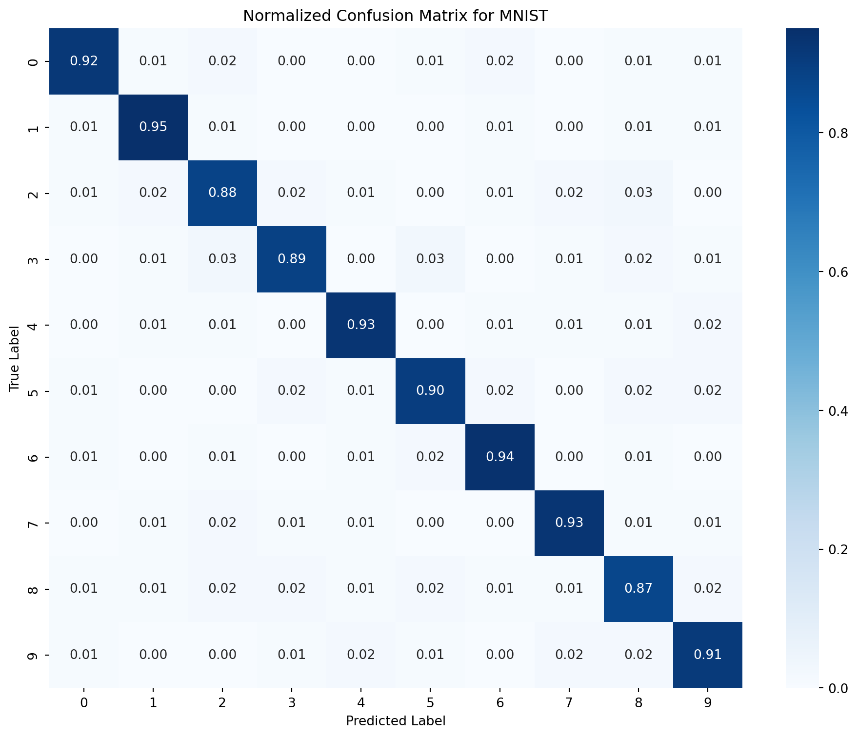
# Simulated confusion matrix for MNIST (normalized)
cm = np.array([
    [0.92, 0.01, 0.02, 0.00, 0.00, 0.01, 0.02, 0.00, 0.01, 0.01],
    [0.01, 0.95, 0.01, 0.00, 0.00, 0.00, 0.01, 0.00, 0.01, 0.01],
    [0.01, 0.02, 0.88, 0.02, 0.01, 0.00, 0.01, 0.02, 0.03, 0.00],
    [0.00, 0.01, 0.03, 0.89, 0.00, 0.03, 0.00, 0.01, 0.02, 0.01],
    [0.00, 0.01, 0.01, 0.00, 0.93, 0.00, 0.01, 0.01, 0.01, 0.02],
    [0.01, 0.00, 0.00, 0.02, 0.01, 0.90, 0.02, 0.00, 0.02, 0.02],
    [0.01, 0.00, 0.01, 0.00, 0.01, 0.02, 0.94, 0.00, 0.01, 0.00],
    [0.00, 0.01, 0.02, 0.01, 0.01, 0.00, 0.00, 0.93, 0.01, 0.01],
    [0.01, 0.01, 0.02, 0.02, 0.01, 0.02, 0.01, 0.01, 0.87, 0.02],
    [0.01, 0.00, 0.00, 0.01, 0.02, 0.01, 0.00, 0.02, 0.02, 0.91]
])

plt.figure(figsize=(10, 8))
sns.heatmap(cm, annot=True, fmt='.2f', cmap='Blues', cbar=True,
            xticklabels=range(10), yticklabels=range(10))
plt.xlabel('Predicted Label')
plt.ylabel('True Label')
plt.title('Normalized Confusion Matrix for MNIST')
plt.tight_layout()
plt.show()

To create a confusion matrix from your model’s predictions:

from sklearn.metrics import confusion_matrix
import numpy as np

def create_confusion_matrix(model, data_loader, device):
    model.eval()
    all_preds = []
    all_labels = []
    
    with torch.no_grad():
        for inputs, labels in data_loader:
            inputs, labels = inputs.to(device), labels.to(device)
            outputs = model(inputs)
            _, preds = torch.max(outputs, 1)
            
            all_preds.extend(preds.cpu().numpy())
            all_labels.extend(labels.cpu().numpy())
    
    # Create confusion matrix
    cm = confusion_matrix(all_labels, all_preds)
    
    # Normalize by row (true labels)
    cm_normalized = cm.astype('float') / cm.sum(axis=1)[:, np.newaxis]
    
    return cm_normalized

The confusion matrix reveals systematic patterns in classification errors. In MNIST, common confusions occur between visually similar digits:

  • 4 and 9 (similar upper structures)
  • 3 and 5 (similar curvature patterns)
  • 7 and 1 (similar straight-line components)

These error patterns typically persist regardless of model architecture, reflecting the inherent visual ambiguity of certain digit pairs rather than limitations specific to the logistic classifier.

2 Fashion MNIST Classification with PyTorch

Fashion MNIST is a dataset of Zalando’s article images consisting of 28×28 grayscale images across 10 fashion categories. Like the original MNIST, it contains 60,000 training images and 10,000 test images, but presents a more challenging classification task than digit recognition.

2.1 Using Built-in Fashion MNIST Dataset

PyTorch provides direct access to the Fashion MNIST dataset through the torchvision package, eliminating the need for custom dataset implementation:

import torch
import torchvision
from torchvision import datasets, transforms

# Define the root directory for data storage
data_root = './data'

# Define transformations
transform = transforms.Compose([
    transforms.ToTensor(),  # Convert PIL Image to tensor and scale values to [0.0, 1.0]
])

# Load Fashion MNIST datasets
train_dataset = datasets.FashionMNIST(
    root=data_root,
    train=True,
    download=True,
    transform=transform
)

test_dataset = datasets.FashionMNIST(
    root=data_root,
    train=False,
    download=True,
    transform=transform
)

The label map for Fashion MNIST is:

label_map = {
    0: 'T-shirt/top',
    1: 'Trouser',
    2: 'Pullover',
    3: 'Dress',
    4: 'Coat',
    5: 'Sandal',
    6: 'Shirt',
    7: 'Sneaker',
    8: 'Bag',
    9: 'Ankle boot'
}

2.2 Transform Pipelines for Image Preprocessing

The transforms module in PyTorch provides tools for preprocessing image data before feeding it to models. Transforms can be composed into pipelines using transforms.Compose.

2.2.1 Common Transforms for Fashion MNIST

# Basic transformation: just convert to tensor
basic_transform = transforms.Compose([
    transforms.ToTensor(),  # Convert to tensor and scale to [0, 1]
])

# More complex transformation
advanced_transform = transforms.Compose([
    transforms.ToTensor(),  # Convert to tensor and scale to [0, 1]
    transforms.Normalize((0.5,), (0.5,)),  # Normalize with mean=0.5, std=0.5 to get [-1, 1]
])

# With data augmentation (for training only)
augmentation_transform = transforms.Compose([
    transforms.RandomHorizontalFlip(),  # Randomly flip images horizontally
    transforms.RandomRotation(10),      # Randomly rotate images by up to 10 degrees
    transforms.ToTensor(),              # Convert to tensor 
    transforms.Normalize((0.5,), (0.5,))  # Normalize
])

2.2.2 Visualizing Transform Pipelines

The following code demonstrates how transformations affect the input images:

Code
import matplotlib.pyplot as plt
import torch
import numpy as np
from PIL import Image
from torchvision import transforms

# Create a simple 4x4 grayscale image
raw_image = np.zeros((4, 4), dtype=np.uint8)
raw_image[1:3, 1:3] = 255  # White square in center
pil_image = Image.fromarray(raw_image)

# Define transforms
transform1 = transforms.Compose([transforms.ToTensor()])
transform2 = transforms.Compose([
    transforms.ToTensor(),
    transforms.Normalize((0.5,), (0.5,))
])

# Apply transforms
tensor1 = transform1(pil_image)
tensor2 = transform2(pil_image)

# Display results
fig, axes = plt.subplots(1, 3, figsize=(12, 4))

# Original image
axes[0].imshow(raw_image, cmap='gray', vmin=0, vmax=255)
axes[0].set_title('Original (uint8, [0, 255])')
axes[0].axis('off')

# ToTensor result
axes[1].imshow(tensor1.squeeze().numpy(), cmap='gray', vmin=0, vmax=1)
axes[1].set_title('ToTensor (float, [0, 1])')
axes[1].axis('off')

# Normalized result
axes[2].imshow(tensor2.squeeze().numpy(), cmap='gray', vmin=-1, vmax=1)
axes[2].set_title('Normalized (float, [-1, 1])')
axes[2].axis('off')

plt.tight_layout()
plt.show()

# Show raw tensor values
print("ToTensor output values:")
print(tensor1.squeeze().numpy())
print("\nNormalized output values:")
print(tensor2.squeeze().numpy())

ToTensor output values:
[[0. 0. 0. 0.]
 [0. 1. 1. 0.]
 [0. 1. 1. 0.]
 [0. 0. 0. 0.]]

Normalized output values:
[[-1. -1. -1. -1.]
 [-1.  1.  1. -1.]
 [-1.  1.  1. -1.]
 [-1. -1. -1. -1.]]

The transformation pipeline processes each image by:

  1. Converting from PIL Image or numpy.ndarray to PyTorch tensor
  2. Scaling pixel values from [0, 255] to [0, 1]
  3. Optionally applying normalization to center the data distribution

For Fashion MNIST, the simple ToTensor() transform is often sufficient, but normalization can improve convergence in some models.

2.3 Dropout Regularization

Dropout is a powerful regularization technique that randomly deactivates neurons during training, forcing the network to develop redundant representations. This prevents co-adaptation of neurons and reduces overfitting.

2.3.1 Dropout Implementation in PyTorch

In PyTorch, dropout is implemented as a layer that can be added to the network:

import torch.nn as nn

# Example structure for a neural network with dropout
class NeuralNetworkWithDropout(nn.Module):
    def __init__(self, input_size, hidden_size, output_size, dropout_rate):
        super(NeuralNetworkWithDropout, self).__init__()
        # Define layers
        self.flatten = nn.Flatten()
        self.fc1 = nn.Linear(input_size, hidden_size)
        self.relu = nn.ReLU()
        self.dropout = nn.Dropout(p=dropout_rate)
        self.fc2 = nn.Linear(hidden_size, output_size)
    
    def forward(self, x):
        # Define forward pass
        x = self.flatten(x)
        x = self.fc1(x)
        x = self.relu(x)
        x = self.dropout(x)  # Apply dropout after activation
        x = self.fc2(x)
        return x

2.3.2 Dropout Functionality

When applied to a layer, dropout:

  • During training: Randomly sets elements of the input tensor to zero with probability p
  • During inference: Scales the output by 1/(1-p) to maintain the expected value

This dual behavior necessitates tracking the model’s mode:

# Set to training mode - dropout active
model.train()
outputs = model(inputs)  # Some neurons will be dropped

# Set to evaluation mode - dropout inactive
model.eval()
outputs = model(inputs)  # All neurons active, outputs scaled

2.3.3 Mathematical Formulation

For an input vector \(\mathbf{x}\) with elements \(x_i\), dropout applies:

During training: \[y_i = \begin{cases} \frac{x_i}{1-p} & \text{with probability } 1-p \\ 0 & \text{with probability } p \end{cases}\]

During inference: \[y_i = x_i\]

The scaling factor \(\frac{1}{1-p}\) during training ensures that the expected value of the output remains the same, maintaining consistent activation levels between training and inference.

2.3.4 Dropout Activation Patterns

The following visualizes how dropout affects activations in a simple network:

Code
import torch
import torch.nn as nn
import matplotlib.pyplot as plt
import numpy as np

# Set random seed for reproducibility
torch.manual_seed(42)

# Create a simple tensor
x = torch.ones(1, 10)  # A batch of 1 sample with 10 features

# Create dropout layers with different rates
dropout_rates = [0.2, 0.5, 0.8]
dropouts = [nn.Dropout(p=rate) for rate in dropout_rates]

# Set to training mode
for dropout in dropouts:
    dropout.train()

# Apply dropout
results = [dropout(x).detach().numpy() for dropout in dropouts]

# Visualize the results
fig, axes = plt.subplots(len(dropout_rates), 1, figsize=(10, 8))

for i, (rate, result) in enumerate(zip(dropout_rates, results)):
    # Create a bar plot
    axes[i].bar(range(10), result[0], color='blue', alpha=0.7)
    axes[i].set_title(f'Dropout Rate: {rate}')
    axes[i].set_xlabel('Neuron Index')
    axes[i].set_ylabel('Activation')
    axes[i].set_ylim(0, 5)  # Set y-limit to accommodate scaling

plt.tight_layout()
plt.show()

# Print the fraction of active neurons and their scaling
for rate, result in zip(dropout_rates, results):
    active = np.count_nonzero(result)
    expected_active = 10 * (1 - rate)
    avg_value = np.mean(result[result > 0])
    expected_scale = 1 / (1 - rate)
    
    print(f"Dropout {rate}: {active} active neurons (expected ~{expected_active:.1f})")
    print(f"           Average value of active neurons: {avg_value:.4f} (expected {expected_scale:.4f})")
    print()

Dropout 0.2: 8 active neurons (expected ~8.0)
           Average value of active neurons: 1.2500 (expected 1.2500)

Dropout 0.5: 5 active neurons (expected ~5.0)
           Average value of active neurons: 2.0000 (expected 2.0000)

Dropout 0.8: 5 active neurons (expected ~2.0)
           Average value of active neurons: 5.0000 (expected 5.0000)

As shown, higher dropout rates lead to:

  1. Fewer active neurons during training
  2. Larger scaling factors for the remaining neurons
  3. Greater stochasticity in the network’s behavior

2.4 Batches and Dimensions in nn.Module

Understanding how tensors flow through a PyTorch model is essential for debugging and optimization. Let’s examine tensor dimensions at each stage of the network:

import torch
import torch.nn as nn

class MLPWithPrints(nn.Module):
    def __init__(self, input_size, hidden_size, output_size):
        super(MLPWithPrints, self).__init__()
        self.flatten = nn.Flatten()
        self.fc1 = nn.Linear(input_size, hidden_size)
        self.relu = nn.ReLU()
        self.fc2 = nn.Linear(hidden_size, output_size)
    
    def forward(self, x):
        print(f"Input shape: {x.shape}")
        
        # Flatten the input
        x = self.flatten(x)
        print(f"After flatten: {x.shape}")
        
        # First linear layer
        x = self.fc1(x)
        print(f"After fc1: {x.shape}")
        
        # ReLU activation
        x = self.relu(x)
        print(f"After ReLU: {x.shape}")
        
        # Second linear layer
        x = self.fc2(x)
        print(f"After fc2: {x.shape}")
        
        return x

# Example tensor dimensions
batch_size = 32
channels = 1  # Grayscale images
height, width = 28, 28  # Fashion MNIST image dimensions

# Create a dummy batch
dummy_input = torch.randn(batch_size, channels, height, width)

The expected output dimensions would be:

Input shape: torch.Size([32, 1, 28, 28])
After flatten: torch.Size([32, 784])
After fc1: torch.Size([32, 128])
After ReLU: torch.Size([32, 128])
After fc2: torch.Size([32, 10])

2.4.1 Batch Dimension Propagation

The batch dimension (the first dimension) is preserved throughout the network. This allows for parallel processing of multiple samples:

  1. Input: [batch_size, channels, height, width]
  2. Flattened: [batch_size, channelsheightwidth]
  3. Linear layers: [batch_size, layer_output_size]
  4. Final output: [batch_size, num_classes]

PyTorch operations are designed to operate on batches, applying the same transformation to each sample in the batch independently.

2.4.2 Verifying Batch Operations

To verify that operations are correctly applied across the batch dimension:

def verify_batch_independence(model, batch_size=2):
    # Create two identical images
    img = torch.randn(1, 28, 28)
    batch1 = torch.stack([img, img])  # Batch with identical images
    
    # Process as a batch
    batch_output = model(batch1)
    
    # Process individually
    individual_outputs = []
    for i in range(batch_size):
        individual_outputs.append(model(img.unsqueeze(0)))
    
    # Compare outputs
    for i in range(batch_size):
        # Check if individual output matches corresponding batch output
        is_equal = torch.allclose(batch_output[i], individual_outputs[i].squeeze(0))
        print(f"Sample {i}: Batch processing identical to individual processing: {is_equal}")

This verification confirms that PyTorch models process each sample in a batch independently, which is a key assumption in mini-batch training.

2.5 Accessing and Analyzing Model Parameters

PyTorch models store learnable parameters (weights and biases) that can be accessed for analysis, visualization, or manipulation.

2.5.1 Accessing All Parameters

To access all parameters of a model:

for name, param in model.named_parameters():
    print(f"Layer: {name}, Shape: {param.shape}, Type: {param.dtype}")

2.5.2 Accessing Parameters of Specific Layers

For a model with named layers, parameters can be accessed directly:

# Access weights of the first linear layer
fc1_weights = model.fc1.weight
fc1_bias = model.fc1.bias

# Access weights of the second linear layer
fc2_weights = model.fc2.weight
fc2_bias = model.fc2.bias

print(f"FC1 weights shape: {fc1_weights.shape}")
print(f"FC1 bias shape: {fc1_bias.shape}")
print(f"FC2 weights shape: {fc2_weights.shape}")
print(f"FC2 bias shape: {fc2_bias.shape}")

2.5.3 Visualizing Weight Distributions

Analyzing weight distributions is essential for understanding the effects of regularization:

import matplotlib.pyplot as plt
import numpy as np

def plot_weight_histograms(model, bins=50):
    """Plot histograms of weights for each layer in the model."""
    # Get weight parameters
    weights = []
    layer_names = []
    
    for name, param in model.named_parameters():
        if 'weight' in name:  # Only plot weights, not biases
            weights.append(param.data.cpu().numpy().flatten())
            layer_names.append(name)
    
    # Create plot
    n_layers = len(weights)
    fig, axes = plt.subplots(n_layers, 1, figsize=(10, 4 * n_layers))
    
    # Handle case of only one layer
    if n_layers == 1:
        axes = [axes]
    
    # Plot histogram for each layer
    for i, (name, w) in enumerate(zip(layer_names, weights)):
        axes[i].hist(w, bins=bins, alpha=0.7)
        axes[i].set_title(f'Weight Distribution - {name}')
        axes[i].set_xlabel('Weight Value')
        axes[i].set_ylabel('Frequency')
        
        # Add statistics
        mean = np.mean(w)
        std = np.std(w)
        axes[i].axvline(mean, color='r', linestyle='dashed', linewidth=1)
        axes[i].text(0.95, 0.95, f'Mean: {mean:.4f}\nStd: {std:.4f}',
                    transform=axes[i].transAxes, ha='right', va='top',
                    bbox=dict(boxstyle='round', facecolor='white', alpha=0.5))
    
    plt.tight_layout()
    return fig

To compare models with different regularization settings:

# Create two models with different structures
# Note: Specific sizes and configurations should be determined based on
# the requirements of your specific problem

# Create models and train them (training code not shown)
# ...

# After training, analyze their weight distributions
def plot_weight_distribution(model, layer_name):
    """Plot histogram of weights for a specific layer."""
    # Get the weights
    if hasattr(model, layer_name):
        weights = getattr(model, layer_name).weight.data.cpu().numpy().flatten()
    else:
        print(f"Layer {layer_name} not found in model")
        return
    
    # Plot histogram
    plt.figure(figsize=(8, 5))
    plt.hist(weights, bins=50, alpha=0.7)
    plt.title(f'Weight Distribution - {layer_name}')
    plt.xlabel('Weight Value')
    plt.ylabel('Frequency')
    plt.grid(True, alpha=0.3)
    plt.show()

2.5.4 Extracting Weight Matrices for Advanced Analysis

For more detailed analysis of weight matrices:

# Get the weight matrix of the first layer
weight_matrix = model.fc1.weight.data.cpu().numpy()

# Reshape to visualize each neuron's incoming connections
plt.figure(figsize=(10, 8))
for i in range(min(9, weight_matrix.shape[0])):  # Show up to 9 neurons
    plt.subplot(3, 3, i+1)
    # Reshape to 28x28 to visualize as an image
    plt.imshow(weight_matrix[i].reshape(28, 28), cmap='viridis')
    plt.title(f'Neuron {i+1}')
    plt.axis('off')
plt.tight_layout()
plt.show()

This visualization reveals what patterns each neuron in the hidden layer has learned to detect in the input images.

2.5.5 Understanding Weight Magnitude Distribution

The effect of L2 regularization and dropout on weight distributions can be quantified:

def compare_weight_statistics(model1, model2, layer_name="fc1.weight"):
    """Compare statistical properties of weights between two models for a specific layer."""
    # Extract weights from the specified layer
    if hasattr(model1, layer_name.split('.')[0]):
        weights1 = getattr(model1, layer_name.split('.')[0]).weight.data.cpu().numpy().flatten()
    else:
        print(f"Layer {layer_name} not found in model1")
        return
        
    if hasattr(model2, layer_name.split('.')[0]):
        weights2 = getattr(model2, layer_name.split('.')[0]).weight.data.cpu().numpy().flatten()
    else:
        print(f"Layer {layer_name} not found in model2")
        return
    
    # Calculate statistics
    stats1 = {
        'mean': np.mean(weights1),
        'std': np.std(weights1),
        'min': np.min(weights1),
        'max': np.max(weights1),
        'l2_norm': np.sqrt(np.sum(np.square(weights1)))
    }
    
    stats2 = {
        'mean': np.mean(weights2),
        'std': np.std(weights2),
        'min': np.min(weights2),
        'max': np.max(weights2),
        'l2_norm': np.sqrt(np.sum(np.square(weights2)))
    }
    
    # Print comparison
    print(f"=== Weight Statistics for {layer_name} ===")
    for stat in stats1.keys():
        print(f"{stat}: {stats1[stat]:.4f} (Model 1) vs {stats2[stat]:.4f} (Model 2)")

Typical effects of regularization on weight distributions include:

  • Reduced L2 norm (weight magnitude) with L2 regularization
  • More weights near zero with L1 regularization
  • Larger variance in weight magnitudes with dropout

3 CIFAR-10 Classification with PyTorch

CIFAR-10 is a dataset of 32×32 color images in 10 classes, with 6,000 images per class (50,000 training images and 10,000 test images). Unlike MNIST and Fashion MNIST, CIFAR-10 contains color images, which introduces additional complexity to the classification task.

3.1 Working with Color Image Data

In PyTorch, color images have an additional channel dimension compared to grayscale images. Understanding this representation is crucial for processing RGB data correctly.

3.1.1 Color Image Representation

Color images in CIFAR-10 have three channels (RGB):

Code
import torch
import torchvision
import torchvision.transforms as transforms
import matplotlib.pyplot as plt
import numpy as np

# Set random seed for reproducibility
torch.manual_seed(42)
np.random.seed(42)

# Load a few CIFAR-10 images to demonstrate color channels
transform = transforms.Compose([transforms.ToTensor()])
cifar_dataset = torchvision.datasets.CIFAR10(root='/Users/brandon/Data/pytorch/data', train=True,
                                             download=True, transform=transform)

# Get a sample image
image, label = cifar_dataset[0]

# Print the shape of the image tensor
print(f"CIFAR-10 image shape: {image.shape}")

# Display the image and its channels
fig, axes = plt.subplots(1, 4, figsize=(16, 4))

# Original RGB image
axes[0].imshow(image.permute(1, 2, 0))  # Change from (C, H, W) to (H, W, C) for plotting
axes[0].set_title('Original RGB Image')
axes[0].axis('off')

# Individual color channels
channel_names = ['Red Channel', 'Green Channel', 'Blue Channel']
for i in range(3):
    # Create a copy with only one channel active
    channel_img = torch.zeros_like(image)
    channel_img[i] = image[i]
    
    # Display the channel
    axes[i+1].imshow(channel_img.permute(1, 2, 0))
    axes[i+1].set_title(channel_names[i])
    axes[i+1].axis('off')

plt.tight_layout()
plt.show()
Files already downloaded and verified
CIFAR-10 image shape: torch.Size([3, 32, 32])

Key differences in tensor shapes for color vs. grayscale:

  • MNIST (grayscale): [batch_size, 1, 28, 28]
  • CIFAR-10 (color): [batch_size, 3, 32, 32]

This affects the input size of the network:

  • MNIST flattened input: 28 × 28 × 1 = 784 features
  • CIFAR-10 flattened input: 32 × 32 × 3 = 3,072 features

3.1.2 Loading CIFAR-10 Dataset

PyTorch’s torchvision package provides direct access to the CIFAR-10 dataset:

import torch
import torchvision
import torchvision.transforms as transforms

# Define transforms
transform = transforms.Compose([
    transforms.ToTensor(),
    transforms.Normalize((0.5, 0.5, 0.5), (0.5, 0.5, 0.5))  # Normalize RGB channels
])

# Load CIFAR-10 datasets with automatic download if needed
train_dataset = torchvision.datasets.CIFAR10(
    root='./data',
    train=True,
    download=True,
    transform=transform
)

test_dataset = torchvision.datasets.CIFAR10(
    root='./data',
    train=False,
    download=True,
    transform=transform
)

# Create data loaders
train_loader = torch.utils.data.DataLoader(
    train_dataset,
    batch_size=100,
    shuffle=True,
    num_workers=2  # Parallel data loading
)

test_loader = torch.utils.data.DataLoader(
    test_dataset,
    batch_size=100,
    shuffle=False,
    num_workers=2
)

# Class labels
classes = ('plane', 'car', 'bird', 'cat', 'deer',
           'dog', 'frog', 'horse', 'ship', 'truck')

Note the differences in the normalization compared to grayscale datasets:

  • For grayscale: transforms.Normalize((0.5,), (0.5,))
  • For RGB: transforms.Normalize((0.5, 0.5, 0.5), (0.5, 0.5, 0.5))

3.1.3 Visualizing CIFAR-10 Images

To better understand the dataset, let’s visualize a batch of images:

Code
# Load CIFAR-10 without normalization for better visualization
cifar_vis_dataset = torchvision.datasets.CIFAR10(
    root='/Users/brandon/Data/pytorch/data',
    train=True,
    download=True,
    transform=transforms.ToTensor()
)

# Define class names
classes = ('plane', 'car', 'bird', 'cat', 'deer',
           'dog', 'frog', 'horse', 'ship', 'truck')

# Function to show images from a single class
def show_class_images(dataset, class_idx, num_images=5):
    fig, axes = plt.subplots(1, num_images, figsize=(15, 3))
    
    # Find images of the specified class
    class_images = []
    for i in range(len(dataset)):
        _, label = dataset[i]
        if label == class_idx:
            class_images.append(i)
            if len(class_images) == num_images:
                break
    
    # Display the images
    for i, idx in enumerate(class_images):
        img, _ = dataset[idx]
        axes[i].imshow(img.permute(1, 2, 0))  # Convert from CHW to HWC format
        axes[i].set_title(f"{classes[class_idx]}")
        axes[i].axis('off')
    
    plt.tight_layout()
    plt.show()

# Show 5 examples of 'airplane' class (index 0)
show_class_images(cifar_vis_dataset, 0)

# Show 5 examples of 'cat' class (index 3)
show_class_images(cifar_vis_dataset, 3)
Files already downloaded and verified

Code
# Show a grid of random images from different classes
def show_random_images(dataset, num_rows=3, num_cols=4):
    fig, axes = plt.subplots(num_rows, num_cols, figsize=(12, 9))
    
    # Get random indices
    indices = np.random.choice(len(dataset), num_rows * num_cols, replace=False)
    
    for i, ax in enumerate(axes.flat):
        img, label = dataset[indices[i]]
        ax.imshow(img.permute(1, 2, 0))  # Convert from CHW to HWC format
        ax.set_title(f"{classes[label]}")
        ax.axis('off')
    
    plt.tight_layout()
    plt.show()

# Show random images
show_random_images(cifar_vis_dataset)

3.2 Overview of PyTorch Datasets

PyTorch offers a variety of built-in datasets through the torchvision, torchaudio, and torchtext packages. These datasets facilitate research and benchmarking by providing standardized implementations of common datasets.

3.2.1 Vision Datasets in torchvision

torchvision provides access to popular computer vision datasets:

Dataset Description Image Size Classes Samples
MNIST Handwritten digits 28×28 (grayscale) 10 70,000
Fashion-MNIST Clothing items 28×28 (grayscale) 10 70,000
CIFAR-10 General objects 32×32 (color) 10 60,000
CIFAR-100 General objects 32×32 (color) 100 60,000
STL10 General objects 96×96 (color) 10 13,000
ImageNet Object recognition Variable (color) 1,000 1.2M
COCO Object detection Variable (color) 80 330K

Loading these datasets follows a similar pattern:

# MNIST
mnist = torchvision.datasets.MNIST(root='./data', train=True, download=True, transform=transform)

# CIFAR-100
cifar100 = torchvision.datasets.CIFAR100(root='./data', train=True, download=True, transform=transform)

# STL10
stl10 = torchvision.datasets.STL10(root='./data', split='train', download=True, transform=transform)

3.2.2 Audio Datasets in torchaudio

PyTorch also provides access to audio datasets through torchaudio:

import torchaudio

# Load example of LIBRISPEECH dataset
librispeech = torchaudio.datasets.LIBRISPEECH(
    root='./data', 
    url='dev-clean', 
    download=True
)

# Load example of SPEECHCOMMANDS dataset
speechcommands = torchaudio.datasets.SPEECHCOMMANDS(
    root='./data', 
    download=True
)

Example of viewing audio data:

Code
# Let's load a small audio sample for visualization
import torchaudio
import matplotlib.pyplot as plt
from IPython.display import Audio

try:
    # Try to load a sample from a small subset of SPEECHCOMMANDS
    # If failed, we'll create a synthetic sample
    dataset = torchaudio.datasets.SPEECHCOMMANDS(
        "/Users/brandon/Data/pytorch/data",
        download=True,
        subset='testing'
    )
    
    # Get the first sample
    waveform, sample_rate, label, _, _ = dataset[0]
    print(f"Audio shape: {waveform.shape}, Sample rate: {sample_rate}, Label: {label}")
    
except Exception as e:
    print(f"Could not load real dataset: {e}")
    print("Creating synthetic audio sample instead...")
    
    # Create a synthetic audio sample
    sample_rate = 16000
    waveform = torch.sin(2 * torch.pi * 440 * torch.arange(sample_rate * 2) / sample_rate)
    waveform = waveform.unsqueeze(0)  # Add channel dimension
    label = "synthetic_tone"

# Plot the waveform
plt.figure(figsize=(10, 4))
plt.plot(waveform[0].numpy())
plt.title(f"Waveform: {label}")
plt.xlabel("Sample")
plt.ylabel("Amplitude")
plt.tight_layout()
plt.show()

# Plot the spectrogram
specgram = torchaudio.transforms.Spectrogram()(waveform)
plt.figure(figsize=(10, 4))
plt.imshow(specgram.log2()[0, :, :].numpy(), aspect='auto', origin='lower')
plt.title(f"Spectrogram: {label}")
plt.xlabel("Frame")
plt.ylabel("Frequency Bin")
plt.colorbar(format='%+2.0f dB')
plt.tight_layout()
plt.show()
Audio shape: torch.Size([1, 16000]), Sample rate: 16000, Label: right

3.2.3 Text Datasets in torchtext

For natural language processing tasks, PyTorch provides torchtext:

from torchtext.datasets import AG_NEWS

# Load AG_NEWS dataset
train_iter = AG_NEWS(split='train')

These diverse datasets across modalities demonstrate PyTorch’s ecosystem for handling different types of data beyond just images.

3.3 Multi-Layer Networks for CIFAR-10

For complex datasets like CIFAR-10, deeper networks with multiple hidden layers typically achieve better performance. When implementing a multi-layer perceptron (MLP) for CIFAR-10, the tensor dimensions change as follows:

3.3.1 Tensor Flow Through Multi-Layer Networks

Starting with the input shape for a batch of CIFAR-10 images: [batch_size, 3, 32, 32]

# Example tensor flow through a multi-layer MLP
import torch.nn as nn

class MultiLayerMLP(nn.Module):
    def __init__(self):
        super(MultiLayerMLP, self).__init__()
        self.flatten = nn.Flatten()
        # Flatten: [batch_size, 3, 32, 32] -> [batch_size, 3*32*32]
        
        # Define network layers
        # ... (implementation depends on specific architecture)
    
    def forward(self, x):
        # Track tensor dimensions through the network
        print(f"Input: {x.shape}")
        
        x = self.flatten(x)
        print(f"After flatten: {x.shape}")
        
        # Forward through remaining layers
        # ...
        
        return x

3.3.2 Impact of Color Channels on Network Size

The addition of color channels significantly increases the input dimensionality, which has several implications:

  1. Increased Parameter Count: Color images require ~3× more input parameters than grayscale
  2. Higher Model Capacity: More parameters provide higher capacity to learn complex features
  3. Greater Risk of Overfitting: Larger networks are more prone to overfitting
  4. Increased Memory Usage: More parameters require more memory

These factors make regularization techniques like dropout and L2 regularization particularly important for CIFAR-10 models.

3.4 Confusion Matrix Analysis for Multi-Class Problems

Analyzing confusion matrices for a 10-class problem like CIFAR-10 requires considering class relationships. Let’s examine how to interpret confusion patterns:

Code
# Generate a synthetic confusion matrix for CIFAR-10
import numpy as np
import seaborn as sns
import matplotlib.pyplot as plt

# Class names for CIFAR-10
class_names = ['plane', 'car', 'bird', 'cat', 'deer', 
               'dog', 'frog', 'horse', 'ship', 'truck']

# Create a synthetic confusion matrix (normalized)
np.random.seed(42)
# Start with a mostly diagonal matrix
cm = np.eye(10) * 0.7
# Add some confusion between semantically similar classes
# Confusion between vehicles (plane, car, ship, truck)
cm[0, 1] = cm[1, 0] = 0.1  # plane-car
cm[0, 8] = cm[8, 0] = 0.1  # plane-ship
cm[1, 9] = cm[9, 1] = 0.1  # car-truck
cm[8, 9] = cm[9, 8] = 0.1  # ship-truck

# Confusion between animals (bird, cat, deer, dog, frog, horse)
cm[2, 3] = cm[3, 2] = 0.1  # bird-cat
cm[3, 5] = cm[5, 3] = 0.15  # cat-dog
cm[4, 7] = cm[7, 4] = 0.1  # deer-horse
cm[5, 4] = cm[4, 5] = 0.05  # dog-deer

# Add some random confusion to make it realistic
noise = np.random.rand(10, 10) * 0.05
cm = cm + noise
# Normalize rows to sum to 1
cm = cm / cm.sum(axis=1, keepdims=True)

# Plot the confusion matrix
plt.figure(figsize=(10, 8))
sns.heatmap(cm, annot=True, fmt='.2f', cmap='Blues', cbar=True,
            xticklabels=class_names, yticklabels=class_names)
plt.xlabel('Predicted')
plt.ylabel('True')
plt.title('Synthetic Confusion Matrix for CIFAR-10')
plt.tight_layout()
plt.show()

3.4.1 Finding Most Confused Classes

To analyze which classes are most confused with each other:

Code
# Function to find most confused classes
def find_most_confused_classes(cm, class_names):
    # Set diagonal elements to 0 to ignore correct classifications
    cm_off_diag = cm.copy()
    np.fill_diagonal(cm_off_diag, 0)
    
    # For each true class, find the most predicted incorrect class
    for i, true_class in enumerate(class_names):
        if np.sum(cm_off_diag[i, :]) > 0:  # Check if there are any confusions
            most_confused_idx = np.argmax(cm_off_diag[i, :])
            confusion_value = cm_off_diag[i, most_confused_idx]
            print(f"True class '{true_class}' is most confused with '{class_names[most_confused_idx]}' ({confusion_value:.2f})")
    
    # Find the two classes that are most confused with each other (highest off-diagonal element)
    max_idx = np.unravel_index(np.argmax(cm_off_diag), cm_off_diag.shape)
    print(f"\nThe two most confused classes overall are '{class_names[max_idx[0]]}' and '{class_names[max_idx[1]]}' "
          f"({cm_off_diag[max_idx]:.2f})")

# Analyze the confusion matrix
find_most_confused_classes(cm, class_names)
True class 'plane' is most confused with 'car' (0.13)
True class 'car' is most confused with 'truck' (0.10)
True class 'bird' is most confused with 'cat' (0.12)
True class 'cat' is most confused with 'dog' (0.16)
True class 'deer' is most confused with 'horse' (0.12)
True class 'dog' is most confused with 'cat' (0.16)
True class 'frog' is most confused with 'truck' (0.05)
True class 'horse' is most confused with 'deer' (0.13)
True class 'ship' is most confused with 'plane' (0.12)
True class 'truck' is most confused with 'car' (0.12)

The two most confused classes overall are 'dog' and 'cat' (0.16)

This type of analysis reveals:

  • Which classes are most difficult for the model to distinguish
  • Potential semantic or visual similarities between classes
  • Areas where the model might need improvement

The confusion patterns in CIFAR-10 often reflect real-world visual similarities:

  • Vehicles (plane, car, ship, truck) may be confused with each other
  • Animals (bird, cat, deer, dog) share visual features that can cause confusion
  • Classes with similar backgrounds or environments may be confused

Understanding these patterns can guide model improvements and provide insights into the dataset’s inherent challenges.