Homework #9 – Getting Started Guide

1 Convolutional Neural Networks

Convolutional neural networks extract spatial features through parameter-sharing operations that exploit local patterns and hierarchical structure in data. Unlike fully connected layers, which require separate parameters for each input-output connection, convolutional layers apply the same set of filters across the input, dramatically reducing parameter count while maintaining spatial awareness.

1.1 How Convolutions Extract Features

The convolution operation in CNNs computes feature maps by sliding filters across the input:

Code

import torch
import torch.nn.functional as F
import matplotlib.pyplot as plt
import numpy as np

# Create a simple input feature map (7x7)
input_feature = torch.zeros(7, 7)
input_feature[2:5, 2:5] = torch.tensor([[1, 2, 1], [0, 1, 0], [1, 0, 1]])

# Create a simple convolutional kernel (3x3)
kernel = torch.tensor([[-1, 0, 1], [-1, 0, 1], [-1, 0, 1]]).float()

# Apply convolution manually to understand the operation
output_manual = torch.zeros(7, 7)

# Compute convolution with zero padding
for i in range(7):
    for j in range(7):
        # 3x3 region centered at (i,j)
        region = torch.zeros(3, 3)
        for ki in range(3):
            for kj in range(3):
                if 0 <= i-1+ki < 7 and 0 <= j-1+kj < 7:
                    region[ki, kj] = input_feature[i-1+ki, j-1+kj]
        # Element-wise multiplication and sum
        output_manual[i, j] = (region * kernel).sum()

# Also use PyTorch's conv2d for comparison
input_tensor = input_feature.unsqueeze(0).unsqueeze(0)  # Add batch and channel dims
kernel_tensor = kernel.unsqueeze(0).unsqueeze(0)  # Add out_channel and in_channel dims
output_torch = F.conv2d(input_tensor, kernel_tensor, padding=1).squeeze()

# Visualization
fig, axes = plt.subplots(1, 4, figsize=(15, 4))

# Display input with values
axes[0].imshow(input_feature, cmap='viridis')
axes[0].set_title('Input Feature Map')
# Add grid lines
for i in range(8):
    axes[0].axhline(i-0.5, color='white', linewidth=1)
    axes[0].axvline(i-0.5, color='white', linewidth=1)
# Add values as text
for i in range(7):
    for j in range(7):
        value = input_feature[i, j].item()
        axes[0].text(j, i, f'{value:.0f}', ha='center', va='center', 
                    color='white' if value > 0.5 else 'black')
axes[0].axis('off')

# Display kernel with values
axes[1].imshow(kernel, cmap='viridis')
axes[1].set_title('Convolutional Kernel\n(Horizontal Edge Detector)')
# Add grid
for i in range(4):
    axes[1].axhline(i-0.5, color='white', linewidth=1)
    axes[1].axvline(i-0.5, color='white', linewidth=1)
# Add values
for i in range(3):
    for j in range(3):
        value = kernel[i, j].item()
        axes[1].text(j, i, f'{value:.0f}', ha='center', va='center', 
                   color='white' if value != 0 else 'black')
axes[1].axis('off')

# Display manual output with values
im = axes[2].imshow(output_manual, cmap='viridis')
axes[2].set_title('Output Feature Map\n(Manual)')
# Add grid
for i in range(8):
    axes[2].axhline(i-0.5, color='white', linewidth=1)
    axes[2].axvline(i-0.5, color='white', linewidth=1)
# Add values for non-zero cells
for i in range(7):
    for j in range(7):
        value = output_manual[i, j].item()
        if abs(value) > 0.001:  # Only show non-zero values
            axes[2].text(j, i, f'{value:.0f}', ha='center', va='center', 
                       color='white' if value < 0 else 'black')
axes[2].axis('off')

# Display PyTorch output
axes[3].imshow(output_torch.detach().numpy(), cmap='viridis')
axes[3].set_title('Output Feature Map\n(PyTorch)')
# Add grid
for i in range(8):
    axes[3].axhline(i-0.5, color='white', linewidth=1)
    axes[3].axvline(i-0.5, color='white', linewidth=1)
# Add values for non-zero cells
for i in range(7):
    for j in range(7):
        value = output_torch[i, j].item()
        if abs(value) > 0.001:  # Only show non-zero values
            axes[3].text(j, i, f'{value:.0f}', ha='center', va='center', 
                       color='white' if value < 0 else 'black')
axes[3].axis('off')

plt.tight_layout()
plt.show()

2D convolution operation with a 3×3 filter applied to a 7×7 input with zero padding.

The figure below illustrates how a single output cell value is computed in the convolution operation by combining the values in the local receptive field:

Code

# Create a visualization of the computation for a single output value
fig, (ax1, ax2) = plt.subplots(1, 2, figsize=(15, 6), gridspec_kw={'width_ratios': [1.2, 1]})

# Define the region of interest
i, j = 3, 3  # Center position of our example

# Create input and kernel for visualization
input_feature = torch.zeros(7, 7)
input_feature[2:5, 2:5] = torch.tensor([[1, 2, 1], [0, 1, 0], [1, 0, 1]])
kernel = torch.tensor([[-1, 0, 1], [-1, 0, 1], [-1, 0, 1]]).float()

# Compute the result for position (i,j)
region = torch.zeros(3, 3)
for ki in range(3):
    for kj in range(3):
        if 0 <= i-1+ki < 7 and 0 <= j-1+kj < 7:
            region[ki, kj] = input_feature[i-1+ki, j-1+kj]
result = (region * kernel).sum().item()

# Left subplot: Input feature map with highlighted region
ax1.imshow(input_feature, cmap='Blues', alpha=0.8)
ax1.set_title('Input Feature Map with Convolution Window', fontsize=14)

# Add grid
for idx in range(8):
    ax1.axhline(idx-0.5, color='gray', linewidth=1, alpha=0.5)
    ax1.axvline(idx-0.5, color='gray', linewidth=1, alpha=0.5)

# Highlight the kernel region
rect = plt.Rectangle((j-1.5, i-1.5), 3, 3, fill=False, edgecolor='red', linewidth=3)
ax1.add_patch(rect)

# Add values to all input cells
for ii in range(7):
    for jj in range(7):
        value = input_feature[ii, jj].item()
        color = 'black' if value < 0.5 else 'white'
        
        # Highlight cells in the kernel region
        if i-1 <= ii <= i+1 and j-1 <= jj <= j+1:
            weight = 'bold'
            fontsize = 12
            # Add a subtle highlight behind text in region
            ax1.add_patch(plt.Rectangle((jj-0.5, ii-0.5), 1, 1, fill=True, 
                                     alpha=0.2, facecolor='red'))
        else:
            weight = 'normal'
            fontsize = 10
            
        ax1.text(jj, ii, f'{value:.0f}', ha='center', va='center', 
               color=color, fontweight=weight, fontsize=fontsize)

# Set proper axis limits
ax1.set_xlim(-0.5, 6.5)
ax1.set_ylim(6.5, -0.5)  # Reverse y-axis to match usual array display
ax1.axis('off')

# Right subplot: Computation details
ax2.axis('off')
ax2.set_title('Convolution Computation for Position (3,3)', fontsize=14)

# Set up the right side with the input region, kernel, and result
gs = fig.add_gridspec(2, 3, width_ratios=[1, 0.3, 1], height_ratios=[1, 1], 
                    right=0.95, left=0.55, wspace=0.1)

# Region (Input) on the left
region_ax = fig.add_subplot(gs[0, 0])
region_ax.imshow(region, cmap='Blues', alpha=0.8)
region_ax.set_title('Input Region', fontsize=12)
for ii in range(3):
    for jj in range(3):
        region_ax.text(jj, ii, f'{region[ii, jj]:.0f}', ha='center', va='center',
                      color='white' if region[ii, jj] > 0.5 else 'black',
                      fontweight='bold')
region_ax.set_xticks([])
region_ax.set_yticks([])

# Kernel on the right
kernel_ax = fig.add_subplot(gs[0, 2])
kernel_ax.imshow(kernel, cmap='coolwarm')
kernel_ax.set_title('Kernel', fontsize=12)
for ii in range(3):
    for jj in range(3):
        kernel_ax.text(jj, ii, f'{kernel[ii, jj]:.0f}', ha='center', va='center',
                     color='white' if abs(kernel[ii, jj]) > 0.5 else 'black',
                     fontweight='bold')
kernel_ax.set_xticks([])
kernel_ax.set_yticks([])

# Multiplication symbol
fig.text(0.75, 0.75, '×', fontsize=24, ha='center', va='center')

# Element-wise product
product_ax = fig.add_subplot(gs[1, :])
element_product = region * kernel
product_ax.imshow(element_product, cmap='coolwarm')
product_ax.set_title('Element-wise Product', fontsize=12)
for ii in range(3):
    for jj in range(3):
        val = element_product[ii, jj].item()
        product_ax.text(jj, ii, f'{val:.0f}', ha='center', va='center',
                       color='white' if abs(val) > 0.5 else 'black',
                       fontweight='bold')
product_ax.set_xticks([])
product_ax.set_yticks([])

# Add the summation formula below
formula_text = f"Output[3,3] = Sum of Product = {result:.0f}"
ax2.text(0.5, 0.05, formula_text, ha='center', va='center', fontsize=14, 
        fontweight='bold', bbox=dict(facecolor='lightyellow', edgecolor='gray', 
                                    boxstyle='round,pad=0.5'))

# Add annotation arrow from input to computation
con = plt.matplotlib.patches.ConnectionPatch(
    xyA=(j, i), xyB=(0.05, 0.5), 
    coordsA="data", coordsB="axes fraction",
    axesA=ax1, axesB=ax2, 
    arrowstyle="->", linewidth=2, color='red'
)
fig.add_artist(con)

plt.tight_layout()
plt.show()

Computing a single output value in a convolution operation.

In PyTorch, convolutions are implemented with the nn.Conv2d (and related) modules, which accept parameters for kernel size, stride, padding, and number of filters. The implementation creates a tensor of filters initialized with random weights that are updated during backpropagation.

For a 2D convolution: \[\text{Output}(i, j) = \sum_m \sum_n \text{Input}(i+m, j+n) \cdot \text{Kernel}(-m, -n)\]

The filter weights detect different features at each layer, with early layers identifying basic edges and later layers combining these into progressively more complex patterns.

1.2 Receptive Fields and Feature Hierarchy

Each neuron in a CNN responds to a portion of the input space called its receptive field. As information flows through deeper layers, the receptive field increases, allowing deeper neurons to integrate information across larger regions of the original input.

Receptive Field Calculation

The theoretical receptive field size for a neuron in layer \(L\) can be calculated as:

\[R_L = R_{L-1} + (K_L - 1) \times \prod_{i=1}^{L-1} S_i\]

Where \(R_L\) is the receptive field size in layer \(L\), \(K_L\) is the kernel size, and \(S_i\) is the stride at layer \(i\).

Code

import matplotlib.pyplot as plt
import matplotlib.patches as patches
import numpy as np

def calc_receptive_field(kernel_sizes, strides):
    """Calculate receptive field size for each layer"""
    assert len(kernel_sizes) == len(strides)
    r = 1  # Initial receptive field (1 pixel)
    receptive_fields = [1]  # Start with the input layer

    for i in range(len(kernel_sizes)):
        r = r + (kernel_sizes[i] - 1) * np.prod(strides[:i], dtype=int)
        receptive_fields.append(r)

    return receptive_fields

# Example: 5 convolutional layers with 3x3 kernels and stride 1
kernel_sizes = [3, 3, 3, 3, 3]
strides = [1, 1, 1, 1, 1]
receptive_fields = calc_receptive_field(kernel_sizes, strides)

# Visualize nested receptive fields on a single grid
layers = ['Input'] + [f'Conv {i+1}' for i in range(len(kernel_sizes))]

# Create grid size based on largest receptive field
grid_size = max(receptive_fields) + 4
center = grid_size // 2

fig, ax = plt.subplots(figsize=(10, 10))

# Create background grid
grid = np.ones((grid_size, grid_size)) * 0.98
ax.imshow(grid, cmap='gray', vmin=0, vmax=1)

# Color palette for different layers (from light to dark)
colors = ['#fee5d9', '#fcae91', '#fb6a4a', '#de2d26', '#a50f15', '#67000d']

# Draw nested receptive fields from largest to smallest
for idx in range(len(receptive_fields) - 1, -1, -1):
    rf = receptive_fields[idx]
    rf_start = center - rf // 2

    # Draw filled rectangle for receptive field
    rect = patches.Rectangle((rf_start - 0.5, rf_start - 0.5), rf, rf,
                             linewidth=2.5, edgecolor='black',
                             facecolor=colors[idx], alpha=0.7)
    ax.add_patch(rect)

    # Add layer label at corner
    label_offset = 0.5
    ax.text(rf_start + label_offset, rf_start + label_offset,
           f'{layers[idx]}\n{rf}×{rf}',
           fontsize=9, fontweight='bold',
           verticalalignment='top',
           bbox=dict(boxstyle='round,pad=0.4', facecolor='white',
                    edgecolor='black', alpha=0.9))

# Draw grid lines
for i in range(grid_size + 1):
    ax.axhline(i - 0.5, color='gray', linewidth=0.5, alpha=0.3)
    ax.axvline(i - 0.5, color='gray', linewidth=0.5, alpha=0.3)

# Mark center neuron
ax.plot(center, center, 'o', markersize=12, markerfacecolor='yellow',
       markeredgecolor='black', markeredgewidth=2, zorder=100)
ax.text(center, center - 1.5, 'Center\nNeuron',
       ha='center', fontsize=9, fontweight='bold')

# Set axis properties
ax.set_xlim(-0.5, grid_size - 0.5)
ax.set_ylim(grid_size - 0.5, -0.5)  # Invert y-axis
ax.set_title('Receptive Field Growth Through Network Layers\n(Each layer sees a larger region of the input)',
            fontsize=12, fontweight='bold', pad=15)
ax.axis('off')

plt.tight_layout()
plt.show()

print(f"Receptive field progression: {' → '.join(f'{rf}×{rf}' for rf in receptive_fields)}")

Receptive field growth through CNN layers with 3×3 filters and stride 1.

Receptive field progression: 1×1 → 3×3 → 5×5 → 7×7 → 9×9 → 11×11

This hierarchical structure creates a natural feature extraction pyramid, with each subsequent layer detecting more abstract patterns:

First layer: Basic features (edges, corners)
Middle layers: Textures and simple shapes
Deep layers: Complex objects and semantic concepts

1.2.1 Receptive Field Growth

A key feature of CNNs is the expansion of the receptive field as depth increases. Techniques to increase receptive field include:

Strided convolutions: Increase step size when sliding the kernel
Pooling layers: Downsampling operations that reduce spatial dimensions
Dilated convolutions: Insert gaps between kernel elements, maintaining resolution while expanding field

The growth of receptive fields enables deep layers to integrate spatial information across large regions, facilitating the recognition of complex patterns.

1.3 Pooling Operations and Dimensionality Reduction

Pooling layers reduce the spatial dimensions of feature maps while retaining important information. This dimensionality reduction serves multiple purposes:

Reduces computational load in subsequent layers
Creates translation invariance for detected features
Combines features from adjacent spatial locations
Expands the receptive field

Code

# Create a feature map
input_feature = torch.zeros(6, 6)
input_feature[1:5, 1:5] = torch.tensor([
    [0.1, 0.5, 0.7, 0.2],
    [0.9, 0.3, 0.1, 0.8],
    [0.2, 0.6, 0.4, 0.5],
    [0.3, 0.1, 0.7, 0.2]
])

# Apply max pooling
input_tensor = input_feature.unsqueeze(0).unsqueeze(0)
max_pooled = F.max_pool2d(input_tensor, kernel_size=2, stride=2).squeeze()

# Apply average pooling
avg_pooled = F.avg_pool2d(input_tensor, kernel_size=2, stride=2).squeeze()

# Visualization
fig, axes = plt.subplots(1, 3, figsize=(15, 5))

# Original feature map with grid
im0 = axes[0].imshow(input_feature, cmap='viridis')
axes[0].set_title('Original Feature Map (6×6)')
# Add grid lines
for i in range(7):
    axes[0].axhline(i-0.5, color='white', linewidth=1)
    axes[0].axvline(i-0.5, color='white', linewidth=1)
    
# Highlight 2x2 pooling regions with thicker lines
for i in range(0, 6, 2):
    # Horizontal lines
    axes[0].axhline(i-0.5, color='yellow', linewidth=3)
    # Vertical lines
    axes[0].axvline(i-0.5, color='yellow', linewidth=3)
        
# Display values in cells
for i in range(6):
    for j in range(6):
        value = input_feature[i, j].item()
        axes[0].text(j, i, f'{value:.1f}', ha='center', va='center', 
                    color='white' if value > 0.4 else 'black')
axes[0].axis('off')

# Max pooled result with grid
im1 = axes[1].imshow(max_pooled, cmap='viridis')
axes[1].set_title('Max Pooling (2×2, stride=2)')
# Add grid
for i in range(4):
    axes[1].axhline(i-0.5, color='white', linewidth=1)
    axes[1].axvline(i-0.5, color='white', linewidth=1)
# Display values
for i in range(3):
    for j in range(3):
        value = max_pooled[i, j].item()
        axes[1].text(j, i, f'{value:.1f}', ha='center', va='center', 
                    color='white' if value > 0.4 else 'black')
axes[1].axis('off')

# Average pooled result with grid
im2 = axes[2].imshow(avg_pooled, cmap='viridis')
axes[2].set_title('Average Pooling (2×2, stride=2)')
# Add grid
for i in range(4):
    axes[2].axhline(i-0.5, color='white', linewidth=1)
    axes[2].axvline(i-0.5, color='white', linewidth=1)
# Display values
for i in range(3):
    for j in range(3):
        value = avg_pooled[i, j].item()
        axes[2].text(j, i, f'{value:.1f}', ha='center', va='center', 
                    color='white' if value > 0.4 else 'black')
axes[2].axis('off')

plt.tight_layout()
plt.show()

Comparison of MaxPooling and AveragePooling operations (2×2 kernel with stride 2)

1.3.1 Common Pooling Types

Max Pooling: Extracts the maximum value from each pooling region, emphasizing the strongest activations. This effectively selects the most prominent features, highlighting edges and textures in early layers.
Average Pooling: Computes the mean of each pooling region, producing smoother feature maps. This preserves more background information and is sometimes preferred in deeper layers.
Global Pooling: Reduces each feature map to a single value, creating a fixed-size output regardless of input dimensions—often used before fully-connected layers.

1.3.2 Alternatives to Pooling

Modern architectures sometimes replace pooling with:

Strided Convolutions: Downsampling through increased stride rather than explicit pooling.
Convolutional Bottlenecks: Reducing channels then expanding with 1×1 convolutions.

These alternatives maintain more information during downsampling but may require more parameters and computation.

1.4 Batch Normalization and Model Stability

Batch normalization stabilizes and accelerates training by normalizing activations across the batch dimension, reducing internal covariate shift and allowing higher learning rates.

For a layer with inputs \(x\) over a mini-batch, batch normalization:

Computes batch mean: \(\mu_B = \frac{1}{m} \sum_{i=1}^{m} x_i\)
Computes batch variance: \(\sigma_B^2 = \frac{1}{m} \sum_{i=1}^{m} (x_i - \mu_B)^2\)
Normalizes inputs: \(\hat{x}_i = \frac{x_i - \mu_B}{\sqrt{\sigma_B^2 + \epsilon}}\)
Scales and shifts: \(y_i = \gamma \hat{x}_i + \beta\)

The parameters \(\gamma\) and \(\beta\) are learned during training, allowing the network to control the normalization as needed.

Code

# Simulate pre-activation values from different layers
np.random.seed(42)
layer1_activations = np.random.normal(0, 1, 1000)  # Well-behaved early layer
layer5_activations = np.random.normal(5, 4, 1000)  # Later layer with shifted activations

# Apply batch normalization manually
def batch_norm(x, gamma=1.0, beta=0.0, eps=1e-5):
    mean = np.mean(x)
    var = np.var(x)
    x_norm = (x - mean) / np.sqrt(var + eps)
    return gamma * x_norm + beta

# Normalize the activations
layer1_norm = batch_norm(layer1_activations)
layer5_norm = batch_norm(layer5_activations)

# Plot distributions
fig, axes = plt.subplots(2, 2, figsize=(12, 8))

# Layer 1 distributions
axes[0, 0].hist(layer1_activations, bins=30, alpha=0.7, color='blue')
axes[0, 0].set_title('Layer 1: Pre-BN Distribution')
axes[0, 0].axvline(np.mean(layer1_activations), color='red', linestyle='dashed', 
                  label=f'Mean: {np.mean(layer1_activations):.2f}')
axes[0, 0].axvline(np.mean(layer1_activations) + np.std(layer1_activations), color='green', 
                  linestyle='dashed', label=f'Std: {np.std(layer1_activations):.2f}')
axes[0, 0].axvline(np.mean(layer1_activations) - np.std(layer1_activations), color='green', 
                  linestyle='dashed')
axes[0, 0].legend()

axes[0, 1].hist(layer1_norm, bins=30, alpha=0.7, color='blue')
axes[0, 1].set_title('Layer 1: Post-BN Distribution')
axes[0, 1].axvline(np.mean(layer1_norm), color='red', linestyle='dashed', 
                  label=f'Mean: {np.mean(layer1_norm):.2f}')
axes[0, 1].axvline(np.mean(layer1_norm) + np.std(layer1_norm), color='green', 
                  linestyle='dashed', label=f'Std: {np.std(layer1_norm):.2f}')
axes[0, 1].axvline(np.mean(layer1_norm) - np.std(layer1_norm), color='green', 
                  linestyle='dashed')
axes[0, 1].legend()

# Layer 5 distributions
axes[1, 0].hist(layer5_activations, bins=30, alpha=0.7, color='orange')
axes[1, 0].set_title('Layer 5: Pre-BN Distribution')
axes[1, 0].axvline(np.mean(layer5_activations), color='red', linestyle='dashed', 
                  label=f'Mean: {np.mean(layer5_activations):.2f}')
axes[1, 0].axvline(np.mean(layer5_activations) + np.std(layer5_activations), color='green', 
                  linestyle='dashed', label=f'Std: {np.std(layer5_activations):.2f}')
axes[1, 0].axvline(np.mean(layer5_activations) - np.std(layer5_activations), color='green', 
                  linestyle='dashed')
axes[1, 0].legend()

axes[1, 1].hist(layer5_norm, bins=30, alpha=0.7, color='orange')
axes[1, 1].set_title('Layer 5: Post-BN Distribution')
axes[1, 1].axvline(np.mean(layer5_norm), color='red', linestyle='dashed', 
                  label=f'Mean: {np.mean(layer5_norm):.2f}')
axes[1, 1].axvline(np.mean(layer5_norm) + np.std(layer5_norm), color='green', 
                  linestyle='dashed', label=f'Std: {np.std(layer5_norm):.2f}')
axes[1, 1].axvline(np.mean(layer5_norm) - np.std(layer5_norm), color='green', 
                  linestyle='dashed')
axes[1, 1].legend()

plt.tight_layout()
plt.show()

Effect of batch normalization on the distribution of activations.

1.4.1 Batch Norm in CNN Architectures

In convolutional networks, batch normalization is typically applied after convolution but before activation:

# Common CNN block with batch normalization
def conv_bn_block(in_channels, out_channels, kernel_size=3, stride=1, padding=1):
    return nn.Sequential(
        nn.Conv2d(in_channels, out_channels, kernel_size, stride, padding),
        nn.BatchNorm2d(out_channels),  # Normalize across batch and spatial dimensions
        nn.ReLU(inplace=True)
    )

When normalizing convolutional features, the statistics are computed across both batch and spatial dimensions for each channel separately.

1.4.2 Benefits of Batch Normalization

Reduces internal covariate shift (distribution changes between layers)
Makes optimization landscape smoother
Adds regularization effect due to batch statistics noise
Enables higher learning rates, accelerating convergence
Reduces sensitivity to initialization

1.4.3 Batch Norm Implementation

PyTorch provides dedicated modules for batch normalization:

nn.BatchNorm1d: For 1D inputs (fully-connected layers)
nn.BatchNorm2d: For 2D inputs (convolutional layers)
nn.BatchNorm3d: For 3D inputs (volumetric convolutions)

During training, these modules track running statistics (mean and variance) to use during inference when batch statistics aren’t available.

1.5 Comparing 1D, 2D, and 3D Convolutions

Convolutional operations can be applied to inputs with different dimensionality, with the number of dimensions referring to how the convolution kernel moves across the input.

Code

# Create visual comparison of convolution types
fig, axes = plt.subplots(1, 3, figsize=(15, 5))

# 1D Convolution illustration
axes[0].set_title("1D Convolution")
# Create an input signal (1D)
x = np.linspace(0, 10, 100)
signal = np.sin(x) + 0.2 * np.sin(4*x)
kernel = np.array([0.2, 0.5, 0.2])  # Simple smoothing kernel

# Plot signal
axes[0].plot(x, signal, 'b-', alpha=0.7, label='Input Signal')
axes[0].set_ylim(-1.5, 1.5)

# Show kernel
axes[0].plot([4, 4.2, 4.4], [1.2, 1.3, 1.2], 'ro-', linewidth=2, markersize=6, label='Kernel')
axes[0].arrow(4.2, 1.3, 0.5, 0, head_width=0.1, head_length=0.1, fc='r', ec='r')

# Calculate and plot output (simplified)
output = np.convolve(signal, kernel, mode='same')
axes[0].plot(x, output, 'g-', label='Output Signal')
axes[0].legend()
axes[0].grid(alpha=0.3)

# 2D Convolution illustration
axes[1].set_title("2D Convolution")
# Create a simple 2D image
image = np.zeros((8, 8))
image[2:6, 2:6] = 1  # Square in the middle

# Create a 2D representation with grid
axes[1].imshow(image, cmap='Blues', alpha=0.7)
for i in range(9):
    axes[1].axhline(i-0.5, color='gray', linestyle='-', alpha=0.3)
    axes[1].axvline(i-0.5, color='gray', linestyle='-', alpha=0.3)

# Highlight kernel position
kernel_pos = [3, 3]
rect = plt.Rectangle((kernel_pos[1]-1.5, kernel_pos[0]-1.5), 3, 3, 
                    fill=False, edgecolor='red', linewidth=2, label='3×3 Kernel')
axes[1].add_patch(rect)
# Show movement direction
axes[1].arrow(kernel_pos[1], kernel_pos[0], 1, 0, head_width=0.3, head_length=0.3, 
             fc='red', ec='red')
axes[1].arrow(kernel_pos[1], kernel_pos[0], 0, 1, head_width=0.3, head_length=0.3, 
             fc='red', ec='red')
axes[1].text(6, 3, "X", color='red', fontsize=12, fontweight='bold')
axes[1].text(3, 6, "Y", color='red', fontsize=12, fontweight='bold')
axes[1].legend(loc='upper right')
axes[1].axis('off')

# 3D Convolution illustration
axes[2].set_title("3D Convolution")
# Create a 3D visualization (simplification)
from mpl_toolkits.mplot3d import Axes3D
from mpl_toolkits.mplot3d.art3d import Poly3DCollection

# Remove the existing 2D axis and create a 3D one
axes[2].remove()
ax3d = fig.add_subplot(1, 3, 3, projection='3d')
ax3d.set_title("3D Convolution")

# Create vertices for a cube
r = [-1, 1]
vertices = [(x, y, z) for x in r for y in r for z in r]
Z = np.zeros((8, 3))
for i, (x, y, z) in enumerate(vertices):
    Z[i] = [x, y, z]

# Create the faces of the cube
faces = [
    [Z[0], Z[1], Z[3], Z[2]],  # Bottom face
    [Z[4], Z[5], Z[7], Z[6]],  # Top face
    [Z[0], Z[1], Z[5], Z[4]],  # Front face
    [Z[2], Z[3], Z[7], Z[6]],  # Back face
    [Z[1], Z[3], Z[7], Z[5]],  # Right face
    [Z[0], Z[2], Z[6], Z[4]]   # Left face
]

# Draw the cube (input volume)
input_cube = Poly3DCollection(faces, alpha=0.25, linewidths=1, edgecolor='b')
input_cube.set_facecolor('blue')
ax3d.add_collection3d(input_cube)

# Draw a smaller cube (kernel) at an offset
kernel_offset = [0.3, 0.3, 0.3]
kernel_faces = []
for face in faces:
    new_face = []
    for vertex in face:
        # Create a smaller kernel cube (0.5 scale) with offset
        scaled_vertex = [v*0.5 + kernel_offset[i] for i, v in enumerate(vertex)]
        new_face.append(scaled_vertex)
    kernel_faces.append(new_face)

kernel_cube = Poly3DCollection(kernel_faces, alpha=0.7, linewidths=1, edgecolor='r')
kernel_cube.set_facecolor('red')
ax3d.add_collection3d(kernel_cube)

# Show kernel movement directions
ax3d.quiver(kernel_offset[0], kernel_offset[1], kernel_offset[2], 
           0.5, 0, 0, color='red', arrow_length_ratio=0.15)
ax3d.quiver(kernel_offset[0], kernel_offset[1], kernel_offset[2], 
           0, 0.5, 0, color='red', arrow_length_ratio=0.15)
ax3d.quiver(kernel_offset[0], kernel_offset[1], kernel_offset[2], 
           0, 0, 0.5, color='red', arrow_length_ratio=0.15)

ax3d.set_xlim([-1.5, 1.5])
ax3d.set_ylim([-1.5, 1.5])
ax3d.set_zlim([-1.5, 1.5])
ax3d.set_xlabel('X')
ax3d.set_ylabel('Y')
ax3d.set_zlabel('Z')
ax3d.text(1.5, 0, 0, "X", color='red')
ax3d.text(0, 1.5, 0, "Y", color='red')
ax3d.text(0, 0, 1.5, "Z", color='red')

# Add a legend-like text
ax3d.text(-1.5, -1.5, 1.5, "Input Volume", color='blue')
ax3d.text(-1.5, -1.5, 1.3, "3×3×3 Kernel", color='red')

plt.tight_layout()
plt.show()

Comparison of 1D, 2D, and 3D convolution operations

1.5.1 1D Convolution

One-dimensional convolutions slide a kernel along a single axis, processing sequential data like time series, audio signals, or text. This makes them ideal for capturing patterns that evolve over a single dimension:

Code

import torch
import torch.nn.functional as F
import matplotlib.pyplot as plt
import numpy as np
from scipy import signal

# Create a more interesting synthetic audio signal
sample_rate = 1000  # Hz
duration = 1  # second
t = np.linspace(0, duration, int(sample_rate * duration), endpoint=False)

# Generate a musical chord with harmonics
fundamental = 100  # Hz
# Create a more complex signal with harmonics and amplitude envelope
audio_signal = np.sin(2 * np.pi * fundamental * t)                    # Fundamental
audio_signal += 0.5 * np.sin(2 * np.pi * 2 * fundamental * t)         # First harmonic
audio_signal += 0.3 * np.sin(2 * np.pi * 3 * fundamental * t)         # Second harmonic
audio_signal += 0.2 * np.sin(2 * np.pi * 4 * fundamental * t)         # Third harmonic
audio_signal += 0.6 * np.sin(2 * np.pi * (fundamental*1.5) * t)       # Musical fifth

# Add amplitude envelope
envelope = 0.5 * (1 + np.sin(2 * np.pi * 1 * t - np.pi/2))
audio_signal = audio_signal * envelope

# Add some percussion-like elements
for i in range(10):
    # Add transients at regular intervals
    center = i * 0.1
    width = 0.005
    percussion = np.exp(-0.5 * ((t - center) / width) ** 2)
    audio_signal += 0.7 * percussion

# Add subtle noise
audio_signal += 0.05 * np.random.randn(len(t))

# Normalize to range [-1, 1]
audio_signal = audio_signal / max(abs(audio_signal))

# Define classic 1D filter shapes
# Low-pass filter - smoothing kernel that keeps low frequencies
# Simple rolling average
kernel_low_pass = np.ones(5)/5
kernel_low_pass = torch.tensor(kernel_low_pass).float()

# High-pass filter - differential kernel that enhances transitions
kernel_high_pass = torch.tensor([-0.2, -0.2, 0.8, -0.2, -0.2]).float()

# Edge detection filter - finds abrupt changes
kernel_edge = torch.tensor([-0.5, 0, 0.5]).float()

# Convert signal to tensor and add batch and channel dimensions
signal_tensor = torch.tensor(audio_signal).float().unsqueeze(0).unsqueeze(0)

# Apply 1D convolution with different kernels
output_low_pass = F.conv1d(signal_tensor, 
                         kernel_low_pass.view(1, 1, -1), 
                         padding=kernel_low_pass.size(0)//2).squeeze()
output_high_pass = F.conv1d(signal_tensor, 
                          kernel_high_pass.view(1, 1, -1), 
                          padding=kernel_high_pass.size(0)//2).squeeze()
output_edge = F.conv1d(signal_tensor, 
                      kernel_edge.view(1, 1, -1), 
                      padding=kernel_edge.size(0)//2).squeeze()

# Create a single-panel figure for the waveforms
fig, axes = plt.subplots(4, 1, figsize=(12, 10), sharex=True)

# Plot original signal with full range
axes[0].plot(t, audio_signal, 'b-', linewidth=1.5)
axes[0].set_title('Original Audio Signal', fontsize=12)
axes[0].set_ylabel('Amplitude')
axes[0].grid(alpha=0.3)
# Remove x-axis limits to show full signal
axes[0].set_xlim(0, 1)

# Plot kernel visualizations with proper styling
kernel_colors = ['green', 'red', 'purple']
kernel_names = ['Low-pass Filter\n(Moving Average)', 'High-pass Filter\n(Transient Enhancer)', 'Edge Detection\n(Differential)']
kernels = [kernel_low_pass, kernel_high_pass, kernel_edge]

# Create a centered x-axis for kernels 
kernel_centers = []
for kernel in kernels:
    half_size = len(kernel) // 2
    x = np.arange(-half_size, half_size + 1)
    if len(x) > len(kernel):  # Adjust if needed for even-sized kernels
        x = x[:-1]
    kernel_centers.append(x)

for i, (kernel, x, name, color) in enumerate(zip(kernels, kernel_centers, kernel_names, kernel_colors)):
    axes[1].plot(x, kernel.numpy(), 
                color=color, linewidth=2.5, 
                marker='o', markersize=8, label=name)

axes[1].set_title('1D Convolution Kernels', fontsize=12)
axes[1].set_ylabel('Weight')
axes[1].set_xlabel('Relative Position')
axes[1].grid(alpha=0.3)
axes[1].legend(loc='upper right', fontsize=10)
axes[1].set_ylim(-0.6, 1.0)  # Set consistent y limits

# Plot filtered signals with full range
outputs = [output_low_pass, output_high_pass]
titles = ['Low-pass Filtered Signal', 'High-pass Filtered Signal']
colors = ['green', 'red']

for i, (output, title, color) in enumerate(zip(outputs, titles, colors)):
    axes[i+2].plot(t, output.numpy(), color=color, linewidth=1.5)
    axes[i+2].set_title(title, fontsize=12)
    axes[i+2].set_ylabel('Amplitude')
    axes[i+2].grid(alpha=0.3)
    axes[i+2].set_xlim(0, 1)  # Show full signal
    
    # Highlight some regions of interest
    if i == 0:  # Low-pass filter - highlight smoothed areas
        for j in range(10):
            center = j * 0.1
            axes[i+2].axvspan(center-0.02, center+0.02, color='green', alpha=0.15)
    elif i == 1:  # High-pass filter - highlight transients
        for j in range(10):
            center = j * 0.1
            axes[i+2].axvspan(center-0.01, center+0.01, color='red', alpha=0.15)

axes[3].set_xlabel('Time (s)')

# Adjust layout
plt.tight_layout()
plt.show()

# Create a new figure for the edge detection and spectrograms
fig, axes = plt.subplots(2, 2, figsize=(15, 10))

# Plot the edge detection result
axes[0, 0].plot(t, output_edge.numpy(), color='purple', linewidth=1.5)
axes[0, 0].set_title('Edge Detection Result', fontsize=12)
axes[0, 0].set_ylabel('Amplitude')
axes[0, 0].set_xlabel('Time (s)')
axes[0, 0].grid(alpha=0.3)
axes[0, 0].set_xlim(0, 1)  # Show full signal
# Highlight edges
for j in range(10):
    center = j * 0.1
    axes[0, 0].axvspan(center-0.005, center+0.005, color='purple', alpha=0.15)

# Helper function for spectrogram with better settings
def plot_spectrogram(ax, audio, sr, title, color_map='viridis'):
    # Use better spectrogram settings
    f, t, Sxx = signal.spectrogram(audio, sr, nperseg=64, noverlap=48, 
                                  window='hamming', scaling='spectrum')
    # Use log scale for better visualization
    im = ax.pcolormesh(t, f, 10 * np.log10(Sxx + 1e-10), 
                     shading='gouraud', cmap=color_map, vmin=-80, vmax=0)
    ax.set_ylabel('Frequency [Hz]')
    ax.set_xlabel('Time [sec]')
    ax.set_title(title, fontsize=12)
    return im

# Create a custom colormap for the spectrograms
original_cmap = plt.cm.viridis
low_pass_cmap = plt.cm.Greens
high_pass_cmap = plt.cm.Reds

# Spectrograms for original, low-pass and high-pass
im1 = plot_spectrogram(axes[0, 1], audio_signal, sample_rate, 'Original Signal Spectrogram')
fig.colorbar(im1, ax=axes[0, 1], label='Power/Frequency (dB/Hz)')

im2 = plot_spectrogram(axes[1, 0], output_low_pass.numpy(), 
                     sample_rate, 'Low-pass Filtered Spectrogram', low_pass_cmap)
fig.colorbar(im2, ax=axes[1, 0], label='Power/Frequency (dB/Hz)')

im3 = plot_spectrogram(axes[1, 1], output_high_pass.numpy(), 
                     sample_rate, 'High-pass Filtered Spectrogram', high_pass_cmap)
fig.colorbar(im3, ax=axes[1, 1], label='Power/Frequency (dB/Hz)')

# Add annotations to highlight key features
axes[0, 1].annotate('Full frequency\nspectrum', xy=(0.5, 300), xytext=(0.3, 400),
                  arrowprops=dict(facecolor='black', shrink=0.05, width=1.5), fontsize=10)

axes[1, 0].annotate('Low frequencies\npreserved', xy=(0.5, 100), xytext=(0.5, 200),
                  arrowprops=dict(facecolor='black', shrink=0.05, width=1.5), fontsize=10)

axes[1, 1].annotate('High frequencies\npreserved', xy=(0.5, 400), xytext=(0.5, 300),
                  arrowprops=dict(facecolor='black', shrink=0.05, width=1.5), fontsize=10)

plt.tight_layout()
plt.show()

1D convolution for audio signal processing

In PyTorch, 1D convolutions work similarly to their 2D counterparts but operate along a single dimension:

# 1D CNN layer for sequence data (e.g., audio, time series, text)
conv1d = nn.Conv1d(in_channels=1, out_channels=16, kernel_size=3, stride=1, padding=1)
# Input shape: [batch_size, channels, sequence_length]
# Output shape: [batch_size, out_channels, sequence_length]

Common applications include:

Audio processing: Detecting patterns in waveforms, speech recognition, and music analysis
Time series analysis: Identifying temporal patterns in financial data, sensor readings, or biological signals
Text processing: Character-level or word-level pattern recognition in natural language processing
Genomic sequence analysis: Finding motifs in DNA or protein sequences

Architecture patterns for 1D CNNs often mirror those for 2D networks with a sequence of convolutional layers followed by pooling operations to progressively extract higher-level features. For audio processing, dilated convolutions are common to capture long-range dependencies without excessive parameter growth.

1.5.2 2D Convolution

Two-dimensional convolutions slide a kernel across height and width dimensions, processing grid-structured data like images:

# 2D CNN layer for image data
conv2d = nn.Conv2d(in_channels=3, out_channels=64, kernel_size=3, stride=1, padding=1)
# Input shape: [batch_size, channels, height, width]
# Output shape: [batch_size, out_channels, height, width]

This is the standard convolution for image processing tasks like classification, detection, and segmentation.

1.5.3 3D Convolution

Three-dimensional convolutions slide a volumetric kernel across depth, height, and width dimensions, processing volumetric data:

# 3D CNN layer for volumetric data
conv3d = nn.Conv3d(in_channels=1, out_channels=16, kernel_size=3, stride=1, padding=1)
# Input shape: [batch_size, channels, depth, height, width]
# Output shape: [batch_size, out_channels, depth, height, width]

Applications include video analysis (where depth represents time), medical imaging (CT, MRI volumes), and 3D point clouds.

1.5.4 Channels vs. Dimensions

Note that the number of input channels is separate from the convolution dimensionality: - 1D convolution can have multiple input channels (e.g., multi-variable time series) - 2D convolution typically has 1 channel (grayscale) or 3 channels (RGB) - 3D convolution can process multi-channel volumetric data

In each case, the convolution operation is performed across all input channels and produces output feature maps where each map combines information from all input channels.

1.6 Inspecting Network Architectures

PyTorch models are hierarchical structures of modules that can be inspected for architectural understanding and debugging.

1.6.1 Basic Model Inspection

The simplest method is printing the model, which shows the module hierarchy:

Code

# Load a pre-trained ResNet-18 model
resnet18 = models.resnet18(pretrained=True)

# Print model structure for basic inspection
print(resnet18)

# Print the first convolutional layer's parameters
print("\nFirst Conv Layer Details:")
print(f"Type: {type(resnet18.conv1)}")
print(f"Kernel size: {resnet18.conv1.kernel_size}")
print(f"Stride: {resnet18.conv1.stride}")
print(f"Padding: {resnet18.conv1.padding}")
print(f"Input channels: {resnet18.conv1.in_channels}")
print(f"Output channels: {resnet18.conv1.out_channels}")
print(f"Parameter count: {sum(p.numel() for p in resnet18.conv1.parameters())}")

# Examine output shape transformation for a sample input
sample_input = torch.randn(1, 3, 224, 224)  # [batch, channels, height, width]
with torch.no_grad():
    output = resnet18.conv1(sample_input)
    print(f"\nInput shape: {sample_input.shape}")
    print(f"Output shape: {output.shape}")

ResNet(
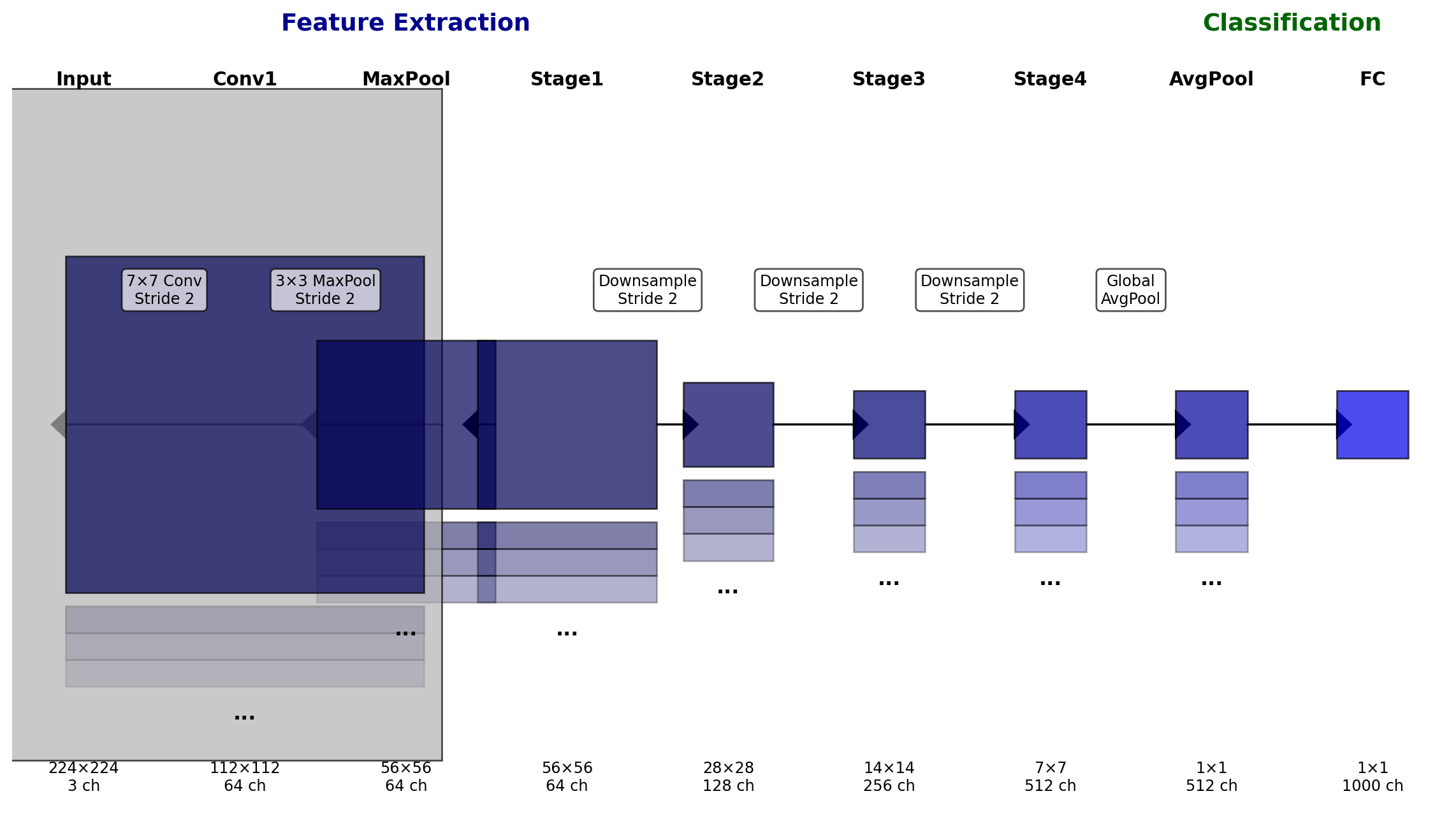
  (conv1): Conv2d(3, 64, kernel_size=(7, 7), stride=(2, 2), padding=(3, 3), bias=False)
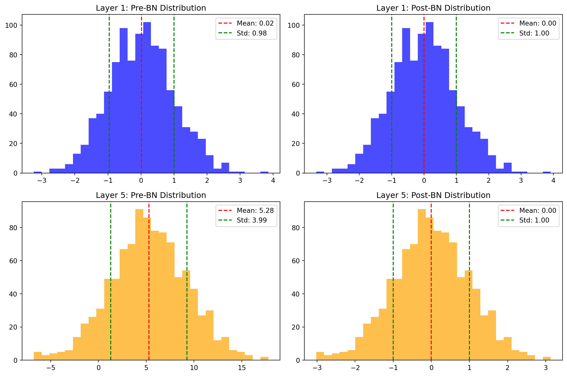
  (bn1): BatchNorm2d(64, eps=1e-05, momentum=0.1, affine=True, track_running_stats=True)
  (relu): ReLU(inplace=True)
  (maxpool): MaxPool2d(kernel_size=3, stride=2, padding=1, dilation=1, ceil_mode=False)
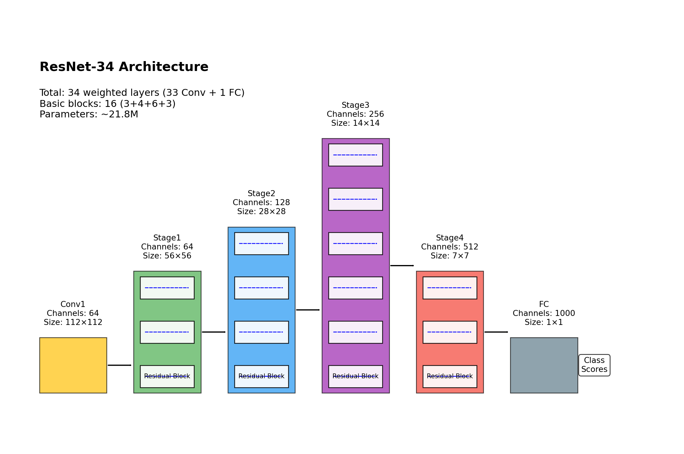
  (layer1): Sequential(
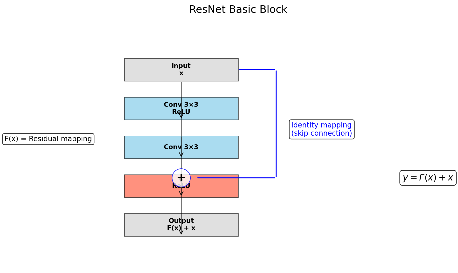
    (0): BasicBlock(
      (conv1): Conv2d(64, 64, kernel_size=(3, 3), stride=(1, 1), padding=(1, 1), bias=False)
      (bn1): BatchNorm2d(64, eps=1e-05, momentum=0.1, affine=True, track_running_stats=True)
      (relu): ReLU(inplace=True)
      (conv2): Conv2d(64, 64, kernel_size=(3, 3), stride=(1, 1), padding=(1, 1), bias=False)
      (bn2): BatchNorm2d(64, eps=1e-05, momentum=0.1, affine=True, track_running_stats=True)
    )
    (1): BasicBlock(
      (conv1): Conv2d(64, 64, kernel_size=(3, 3), stride=(1, 1), padding=(1, 1), bias=False)
      (bn1): BatchNorm2d(64, eps=1e-05, momentum=0.1, affine=True, track_running_stats=True)
      (relu): ReLU(inplace=True)
      (conv2): Conv2d(64, 64, kernel_size=(3, 3), stride=(1, 1), padding=(1, 1), bias=False)
      (bn2): BatchNorm2d(64, eps=1e-05, momentum=0.1, affine=True, track_running_stats=True)
    )
  )
  (layer2): Sequential(
    (0): BasicBlock(
      (conv1): Conv2d(64, 128, kernel_size=(3, 3), stride=(2, 2), padding=(1, 1), bias=False)
      (bn1): BatchNorm2d(128, eps=1e-05, momentum=0.1, affine=True, track_running_stats=True)
      (relu): ReLU(inplace=True)
      (conv2): Conv2d(128, 128, kernel_size=(3, 3), stride=(1, 1), padding=(1, 1), bias=False)
      (bn2): BatchNorm2d(128, eps=1e-05, momentum=0.1, affine=True, track_running_stats=True)
      (downsample): Sequential(
        (0): Conv2d(64, 128, kernel_size=(1, 1), stride=(2, 2), bias=False)
        (1): BatchNorm2d(128, eps=1e-05, momentum=0.1, affine=True, track_running_stats=True)
      )
    )
    (1): BasicBlock(
      (conv1): Conv2d(128, 128, kernel_size=(3, 3), stride=(1, 1), padding=(1, 1), bias=False)
      (bn1): BatchNorm2d(128, eps=1e-05, momentum=0.1, affine=True, track_running_stats=True)
      (relu): ReLU(inplace=True)
      (conv2): Conv2d(128, 128, kernel_size=(3, 3), stride=(1, 1), padding=(1, 1), bias=False)
      (bn2): BatchNorm2d(128, eps=1e-05, momentum=0.1, affine=True, track_running_stats=True)
    )
  )
  (layer3): Sequential(
    (0): BasicBlock(
      (conv1): Conv2d(128, 256, kernel_size=(3, 3), stride=(2, 2), padding=(1, 1), bias=False)
      (bn1): BatchNorm2d(256, eps=1e-05, momentum=0.1, affine=True, track_running_stats=True)
      (relu): ReLU(inplace=True)
      (conv2): Conv2d(256, 256, kernel_size=(3, 3), stride=(1, 1), padding=(1, 1), bias=False)
      (bn2): BatchNorm2d(256, eps=1e-05, momentum=0.1, affine=True, track_running_stats=True)
      (downsample): Sequential(
        (0): Conv2d(128, 256, kernel_size=(1, 1), stride=(2, 2), bias=False)
        (1): BatchNorm2d(256, eps=1e-05, momentum=0.1, affine=True, track_running_stats=True)
      )
    )
    (1): BasicBlock(
      (conv1): Conv2d(256, 256, kernel_size=(3, 3), stride=(1, 1), padding=(1, 1), bias=False)
      (bn1): BatchNorm2d(256, eps=1e-05, momentum=0.1, affine=True, track_running_stats=True)
      (relu): ReLU(inplace=True)
      (conv2): Conv2d(256, 256, kernel_size=(3, 3), stride=(1, 1), padding=(1, 1), bias=False)
      (bn2): BatchNorm2d(256, eps=1e-05, momentum=0.1, affine=True, track_running_stats=True)
    )
  )
  (layer4): Sequential(
    (0): BasicBlock(
      (conv1): Conv2d(256, 512, kernel_size=(3, 3), stride=(2, 2), padding=(1, 1), bias=False)
      (bn1): BatchNorm2d(512, eps=1e-05, momentum=0.1, affine=True, track_running_stats=True)
      (relu): ReLU(inplace=True)
      (conv2): Conv2d(512, 512, kernel_size=(3, 3), stride=(1, 1), padding=(1, 1), bias=False)
      (bn2): BatchNorm2d(512, eps=1e-05, momentum=0.1, affine=True, track_running_stats=True)
      (downsample): Sequential(
        (0): Conv2d(256, 512, kernel_size=(1, 1), stride=(2, 2), bias=False)
        (1): BatchNorm2d(512, eps=1e-05, momentum=0.1, affine=True, track_running_stats=True)
      )
    )
    (1): BasicBlock(
      (conv1): Conv2d(512, 512, kernel_size=(3, 3), stride=(1, 1), padding=(1, 1), bias=False)
      (bn1): BatchNorm2d(512, eps=1e-05, momentum=0.1, affine=True, track_running_stats=True)
      (relu): ReLU(inplace=True)
      (conv2): Conv2d(512, 512, kernel_size=(3, 3), stride=(1, 1), padding=(1, 1), bias=False)
      (bn2): BatchNorm2d(512, eps=1e-05, momentum=0.1, affine=True, track_running_stats=True)
    )
  )
  (avgpool): AdaptiveAvgPool2d(output_size=(1, 1))
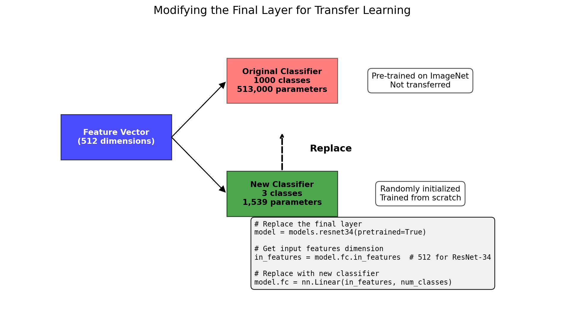
  (fc): Linear(in_features=512, out_features=1000, bias=True)
)

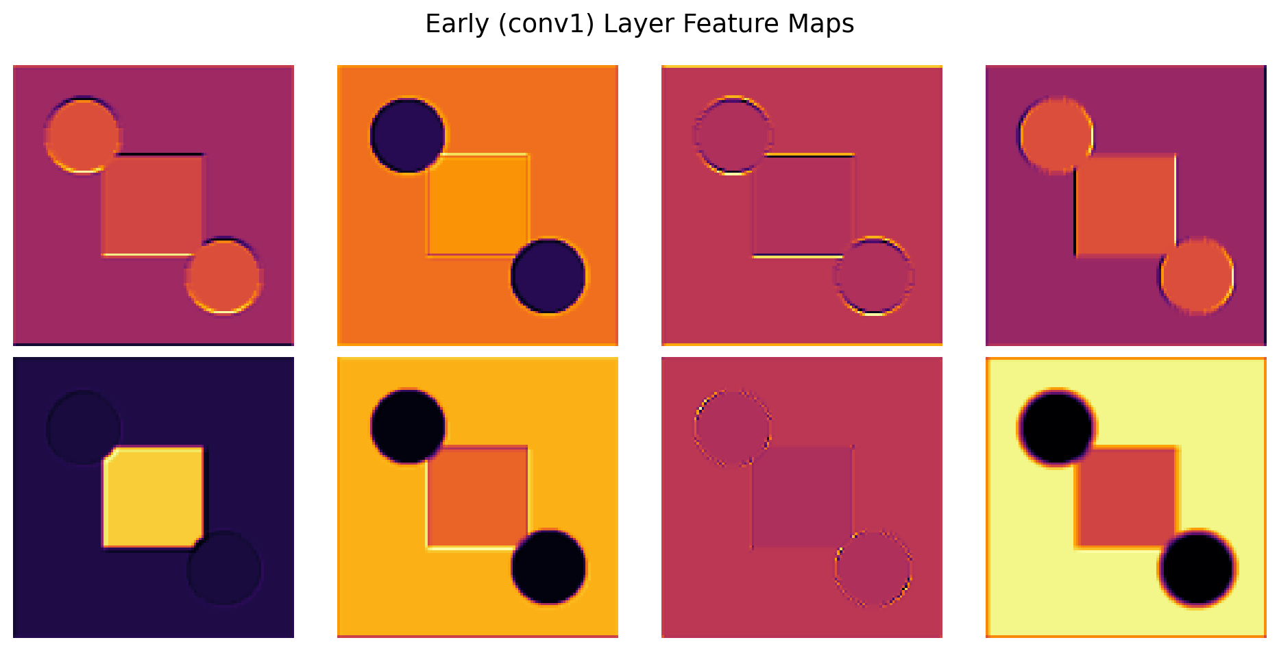
First Conv Layer Details:
Type: <class 'torch.nn.modules.conv.Conv2d'>
Kernel size: (7, 7)
Stride: (2, 2)
Padding: (3, 3)
Input channels: 3
Output channels: 64
Parameter count: 9408

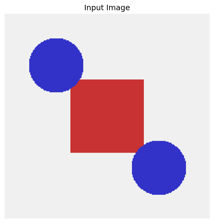
Input shape: torch.Size([1, 3, 224, 224])
Output shape: torch.Size([1, 64, 112, 112])

1.6.2 Advanced Model Analysis

For more detailed inspection, modules can be enumerated to access specific layers:

Code

# Function to count parameters in a model
def count_parameters(model):
    return sum(p.numel() for p in model.parameters() if p.requires_grad)

# Analyze the model structure
layer_types = {}
parameter_counts = {}

for name, module in resnet18.named_modules():
    layer_type = module.__class__.__name__
    if layer_type in layer_types:
        layer_types[layer_type] += 1
    else:
        layer_types[layer_type] = 1
    
    # Count parameters for each layer type
    params = sum(p.numel() for p in module.parameters() if p.requires_grad and p is not None)
    if layer_type in parameter_counts:
        parameter_counts[layer_type] += params
    else:
        parameter_counts[layer_type] = params

# Remove duplicates (parent modules contain child parameters)
for layer_type in list(parameter_counts.keys()):
    if layer_type in ['Sequential', 'ResNet', 'BasicBlock']:
        parameter_counts[layer_type] = 0

# Filter and display layer type distribution
layer_types_filtered = {k: v for k, v in layer_types.items() if v > 0 and k not in ['Sequential', 'ResNet', 'ModuleList']}
parameters_filtered = {k: v for k, v in parameter_counts.items() if v > 0}

print("Layer Type Distribution:")
print("-" * 50)
for layer_type, count in sorted(layer_types_filtered.items(), key=lambda x: -x[1]):
    params = parameters_filtered.get(layer_type, 0)
    print(f"{layer_type:20s}: {count:3d} layers, {params:12,d} parameters")

print("\n" + "=" * 50)
total_params = count_parameters(resnet18)
print(f"Total trainable parameters: {total_params:,}")

Layer Type Distribution:
--------------------------------------------------
Conv2d              :  20 layers,   11,166,912 parameters
BatchNorm2d         :  20 layers,        9,600 parameters
ReLU                :   9 layers,            0 parameters
BasicBlock          :   8 layers,            0 parameters
MaxPool2d           :   1 layers,            0 parameters
AdaptiveAvgPool2d   :   1 layers,            0 parameters
Linear              :   1 layers,      513,000 parameters

==================================================
Total trainable parameters: 11,689,512

1.6.3 Forward Hook Introspection

PyTorch’s hook mechanism provides a powerful way to extract intermediate activations during forward passes:

Code

# Create a function to register forward hooks on selected layers
def get_activation(name, activation_dict):
    def hook(module, input, output):
        activation_dict[name] = output.detach().cpu()
    return hook

# Create a dictionary to store activations
activations = {}

# Register hooks for layers we want to inspect
resnet18.conv1.register_forward_hook(get_activation('conv1', activations))
resnet18.layer1[0].conv1.register_forward_hook(get_activation('layer1.0.conv1', activations))
resnet18.layer2[0].conv1.register_forward_hook(get_activation('layer2.0.conv1', activations))

# Set model to evaluation mode
resnet18.eval()

# Create a more interesting input (checkerboard pattern)
sample_input = torch.zeros(1, 3, 224, 224)
for i in range(224):
    for j in range(224):
        if (i // 28) % 2 == (j // 28) % 2:
            sample_input[0, :, i, j] = 1.0

# Forward pass
with torch.no_grad():
    _ = resnet18(sample_input)

# Visualize some feature maps
fig, axes = plt.subplots(3, 4, figsize=(16, 12))
fig.suptitle('Feature Map Activations', fontsize=16)

# Display input image
axes[0, 0].imshow(sample_input[0].permute(1, 2, 0).cpu().numpy())
axes[0, 0].set_title('Input Image')
axes[0, 0].axis('off')

# Display feature maps from each layer
for i, layer_name in enumerate(['conv1', 'layer1.0.conv1', 'layer2.0.conv1']):
    feature_map = activations[layer_name][0]
    num_filters = min(3, feature_map.size(0))
    
    # Display layer name in first column
    if i > 0:
        axes[i, 0].text(0.5, 0.5, layer_name, 
                      horizontalalignment='center', verticalalignment='center',
                      transform=axes[i, 0].transAxes, fontsize=12)
        axes[i, 0].axis('off')
    
    # Display feature maps
    for j in range(num_filters):
        ax = axes[i, j+1]
        fm = feature_map[j].numpy()
        im = ax.imshow(fm, cmap='viridis')
        ax.set_title(f'Filter {j+1}')
        ax.axis('off')
        fig.colorbar(im, ax=ax, fraction=0.046, pad=0.04)

plt.tight_layout()
plt.subplots_adjust(top=0.9)
plt.show()

Visualizing feature map activations using forward hooks

This hook-based inspection is particularly valuable for: - Debugging network behavior - Visualizing learned features - Understanding how information flows through the network - Identifying dead neurons or saturation issues

1.7 Padding in Convolutional Networks

Padding refers to adding extra pixels around the input’s border before applying convolution. This technique serves several critical purposes in convolutional network design.

1.7.1 Purpose of Padding

The most fundamental reason for padding is to preserve spatial dimensions. Without padding, each convolution operation reduces the output size, causing feature maps to shrink with each layer:

Code

import torch
import torch.nn.functional as F
import matplotlib.pyplot as plt
import numpy as np

# Create a simple input (8x8)
input_feature = torch.zeros(8, 8)
input_feature[2:6, 2:6] = 1.0  # Center square

# Apply 3x3 convolution without padding
kernel = torch.ones(3, 3) / 9.0  # Simple averaging filter

# Add batch and channel dimensions
input_tensor = input_feature.unsqueeze(0).unsqueeze(0)
kernel_tensor = kernel.unsqueeze(0).unsqueeze(0)

# No padding (valid)
output_valid = F.conv2d(input_tensor, kernel_tensor, padding=0).squeeze()

# Create visualization
fig, (ax1, ax2) = plt.subplots(1, 2, figsize=(10, 4))

# Display input with grid
ax1.imshow(input_feature, cmap='viridis')
ax1.set_title('Original Input (8×8)')
for i in range(9):
    ax1.axhline(i-0.5, color='white', linewidth=1)
    ax1.axvline(i-0.5, color='white', linewidth=1)
ax1.axis('off')

# Display output with grid
ax2.imshow(output_valid, cmap='viridis')
ax2.set_title(f'After 3×3 Convolution\nNo Padding (6×6)')
for i in range(7):
    ax2.axhline(i-0.5, color='white', linewidth=1)
    ax2.axvline(i-0.5, color='white', linewidth=1)
ax2.axis('off')

plt.tight_layout()
plt.show()

Effect of convolution without padding: spatial dimensions shrink

The image above demonstrates how a 3×3 convolution without padding reduces an 8×8 input to a 6×6 output. This dimension reduction occurs with each convolutional layer, limiting the potential depth of the network.

Besides maintaining spatial dimensions, padding serves two other important functions:

Preserving border information: Edge pixels appear in fewer convolution operations without padding, giving them less influence on the output
Enabling precise output control: Allows the designer to dictate the exact output dimensions needed for network architecture

1.7.2 Common Padding Strategies

There are three standard approaches to padding:

Code

# Create simple input with a distinct pattern
sample = torch.zeros(8, 8)
sample[2:6, 2:6] = torch.tensor([
    [0.3, 0.5, 0.7, 0.4],
    [0.2, 0.9, 0.8, 0.3],
    [0.4, 0.7, 0.9, 0.2],
    [0.3, 0.4, 0.5, 0.1]
])

# Input with batch and channel dimensions
sample_tensor = sample.unsqueeze(0).unsqueeze(0)

# Apply convolution with different padding strategies
kernel = torch.ones(3, 3) / 9.0  # Simple averaging filter
kernel_tensor = kernel.unsqueeze(0).unsqueeze(0)

# No padding (valid)
output_valid = F.conv2d(sample_tensor, kernel_tensor, padding=0).squeeze()

# Same padding
output_same = F.conv2d(sample_tensor, kernel_tensor, padding=1).squeeze()

# Full padding
input_padded = F.pad(sample_tensor, (2, 2, 2, 2), mode='constant', value=0)
output_full = F.conv2d(input_padded, kernel_tensor, padding=0).squeeze()

# Visualization
fig, axes = plt.subplots(2, 2, figsize=(10, 8))

# Original input
axes[0, 0].imshow(sample, cmap='viridis')
axes[0, 0].set_title('Original Input (8×8)')
for i in range(9):
    axes[0, 0].axhline(i-0.5, color='white', linewidth=1)
    axes[0, 0].axvline(i-0.5, color='white', linewidth=1)
axes[0, 0].axis('off')

# No padding (valid)
axes[0, 1].imshow(output_valid, cmap='viridis')
axes[0, 1].set_title('No Padding ("valid")\nOutput: 6×6')
for i in range(7):
    axes[0, 1].axhline(i-0.5, color='white', linewidth=1)
    axes[0, 1].axvline(i-0.5, color='white', linewidth=1)
axes[0, 1].axis('off')

# Same padding
axes[1, 0].imshow(output_same, cmap='viridis')
axes[1, 0].set_title('Same Padding (p=1)\nOutput: 8×8')
for i in range(9):
    axes[1, 0].axhline(i-0.5, color='white', linewidth=1)
    axes[1, 0].axvline(i-0.5, color='white', linewidth=1)
axes[1, 0].axis('off')

# Full padding
axes[1, 1].imshow(output_full, cmap='viridis')
axes[1, 1].set_title('Full Padding (p=2)\nOutput: 10×10')
for i in range(11):
    axes[1, 1].axhline(i-0.5, color='white', linewidth=1)
    axes[1, 1].axvline(i-0.5, color='white', linewidth=1)
axes[1, 1].axis('off')

plt.tight_layout()
plt.show()

Comparison of padding strategies: no padding, same padding, and full padding

Valid Padding (No Padding):
- No padding is added; output size shrinks with each layer
- Output size: \(O = \lfloor (I - K + 1) / S \rfloor\)
- Used when downsampling is desired or in early CNNs like LeNet
Same Padding:
- Adds padding to keep output dimensions equal to input dimensions (when stride=1)
- Padding amount: \(P = (K - 1) / 2\) (for odd kernel sizes)
- Most commonly used in modern architectures like ResNet
Full Padding:
- Adds padding such that the kernel touches each input pixel in every valid position
- Padding amount: \(P = K - 1\)
- Output size: \(O = I + K - 1\) (when stride=1)

1.7.3 Padding Modes

When applying padding, there are multiple ways to determine what values to place in the padded regions:

Code

# Create a sample input with a gradient pattern
sample = torch.zeros(8, 8)
# Add a gradient pattern
for i in range(8):
    for j in range(8):
        sample[i, j] = 0.7 * (i/7) + 0.3 * (j/7)

# Apply different padding modes
padding_size = 2
modes = ['constant', 'reflect', 'replicate', 'circular']

fig, axes = plt.subplots(2, 2, figsize=(10, 8))
axes = axes.flatten()

# Display different padding types
for i, mode in enumerate(modes):
    padded = F.pad(sample.unsqueeze(0).unsqueeze(0), 
                  (padding_size, padding_size, padding_size, padding_size), 
                  mode=mode, value=0.0).squeeze()
    axes[i].imshow(padded, cmap='viridis')
    axes[i].set_title(f'Padding Mode: {mode}')
    
    # Draw grid lines
    for j in range(padded.shape[0] + 1):
        axes[i].axhline(j-0.5, color='white', linewidth=1)
        axes[i].axvline(j-0.5, color='white', linewidth=1)
    
    # Draw a rectangle showing the original input area
    rect = plt.Rectangle((padding_size-0.5, padding_size-0.5), 8, 8, 
                       fill=False, edgecolor='red', linestyle='-', linewidth=2)
    axes[i].add_patch(rect)
    axes[i].axis('off')

plt.tight_layout()
plt.show()

Different padding modes and their effect on boundary handling

Zero Padding ('constant', value=0):
- Pads with zeros (default)
- Simple but can create artificial edges at boundaries
Reflection Padding ('reflect'):
- Pads by reflecting input content at boundaries
- Better for preserving edge statistics and avoiding boundary artifacts
Replication Padding ('replicate'):
- Extends edge values outward
- Maintains edge continuity well
Circular Padding ('circular'):
- Wraps around (periodic boundary conditions)
- Useful for data with repeating patterns or when simulating infinite fields

Tip

Reflection padding often performs better than zero-padding for image tasks because it reduces artificial boundary effects, especially for larger kernel sizes. This can be particularly important in deeper networks.

1.7.4 Impact on Receptive Field and Network Depth

The padding strategy directly affects how deep a network can be:

Without padding: In a network with kernel size K and no padding, the spatial dimensions will shrink by (K-1) with each layer, limiting maximum depth
With same padding: Networks can reach arbitrary depth while maintaining spatial dimensions, which is why padding is essential for very deep architectures like ResNet

In PyTorch, padding can be specified in two ways:

# 1. As a parameter to convolutional layers
conv = nn.Conv2d(in_channels=3, out_channels=64, kernel_size=3, padding=1)

# 2. As a separate operation
padded_input = F.pad(input, pad=(1, 1, 1, 1), mode='reflect')

1.8 Understanding Kernel Sizes and Output Dimensions

Calculating the output dimensions of convolutional layers is fundamental for designing architectures. The output size depends on input dimensions, kernel size, stride, padding, and dilation:

\[O = \left\lfloor \frac{I + 2P - D(K-1) - 1}{S} \right\rfloor + 1\]

Where: - \(O\): Output dimension - \(I\): Input dimension - \(K\): Kernel size - \(P\): Padding - \(S\): Stride - \(D\): Dilation

Code

def compute_output_size(input_size, kernel_size, stride=1, padding=0, dilation=1):
    """Compute output size of a convolutional layer"""
    return int((input_size + 2*padding - dilation*(kernel_size-1) - 1) / stride + 1)

# Define parameters to explore
input_size = 32
kernel_sizes = [1, 3, 5, 7]
strides = [1, 2]
paddings = [0, 1, 'same']  # 'same' means output size = input size

# Create a grid of combinations
fig, axes = plt.subplots(len(paddings), len(strides), figsize=(12, 9), sharey=True)
fig.suptitle('Output Size vs. Kernel Size', fontsize=16)

for i, padding in enumerate(paddings):
    for j, stride in enumerate(strides):
        ax = axes[i, j]
        output_sizes = []
        
        for kernel_size in kernel_sizes:
            if padding == 'same':
                # Calculate padding needed to keep output same as input
                padding_val = int((kernel_size - 1) / 2)
                output_size = compute_output_size(input_size, kernel_size, stride, padding_val)
            else:
                output_size = compute_output_size(input_size, kernel_size, stride, padding)
            output_sizes.append(output_size)
        
        ax.plot(kernel_sizes, output_sizes, 'o-', linewidth=2, markersize=8)
        ax.set_xlabel('Kernel Size')
        if j == 0:
            ax.set_ylabel('Output Size')
        
        padding_name = f"Padding={padding}" if padding != 'same' else "Padding='same'"
        ax.set_title(f"Stride={stride}, {padding_name}")
        ax.grid(True, alpha=0.3)
        ax.set_xticks(kernel_sizes)
        
        # Add text labels
        for k, (x, y) in enumerate(zip(kernel_sizes, output_sizes)):
            ax.text(x, y+0.5, f"{y}", ha='center', va='bottom')

plt.tight_layout()
plt.subplots_adjust(top=0.9)
plt.show()

Output dimension changes for different convolutional parameters

1.8.1 Parameter Count Calculation

The number of parameters in a convolutional layer depends on the kernel size, input channels, output channels, and whether a bias is used:

\[P = C_{out} \times (C_{in} \times K_h \times K_w + 1)\]

Where: - \(P\): Number of parameters - \(C_{out}\): Number of output channels (filters) - \(C_{in}\): Number of input channels - \(K_h, K_w\): Kernel height and width - The +1 term accounts for bias per output channel

Code

def conv_params(in_channels, out_channels, kernel_size, bias=True):
    """Calculate number of parameters in a convolutional layer"""
    if isinstance(kernel_size, int):
        kernel_size = (kernel_size, kernel_size)
    params = out_channels * (in_channels * kernel_size[0] * kernel_size[1])
    if bias:
        params += out_channels
    return params

# Define parameter ranges
in_channels_list = [3, 64, 128, 256]
out_channels = 64
kernel_sizes = [1, 3, 5, 7]

# Calculate parameters
params_data = []
for in_channels in in_channels_list:
    params_row = []
    for kernel_size in kernel_sizes:
        params_row.append(conv_params(in_channels, out_channels, kernel_size))
    params_data.append(params_row)

# Create a heatmap
fig, ax = plt.subplots(figsize=(10, 8))
im = ax.imshow(params_data, cmap='viridis')

# Add axis labels and title
ax.set_xticks(np.arange(len(kernel_sizes)))
ax.set_yticks(np.arange(len(in_channels_list)))
ax.set_xticklabels([f"{k}×{k}" for k in kernel_sizes])
ax.set_yticklabels([f"{c}" for c in in_channels_list])
ax.set_xlabel('Kernel Size')
ax.set_ylabel('Input Channels')
ax.set_title(f'Parameter Count for Conv2d Layer with {out_channels} Output Channels')

# Add text annotations
for i in range(len(in_channels_list)):
    for j in range(len(kernel_sizes)):
        text = ax.text(j, i, f"{params_data[i][j]:,}", 
                     ha="center", va="center", 
                     color="white" if params_data[i][j] > 50000 else "black")

plt.colorbar(im, label='Parameter Count')
plt.tight_layout()
plt.show()

Parameter count for different convolutional configurations

Understanding these relationships allows for intentional network design that balances computational complexity, parameter efficiency, and representational capacity.

1.9 The Feature Extractor and Classifier Pattern

Deep convolutional networks follow a feature extractor-classifier pattern, with early layers extracting spatial features and later layers performing classification based on these features:

Code

# Create a diagram of feature extractor-classifier pattern
fig, ax = plt.subplots(figsize=(12, 6))

# Define the positions
extractor_start = 0
extractor_width = 6
classifier_width = 3
total_width = extractor_width + classifier_width
height = 2

# Create the main boxes
extractor_rect = plt.Rectangle((extractor_start, 0), extractor_width, height, 
                            fill=True, color='skyblue', alpha=0.7)
classifier_rect = plt.Rectangle((extractor_start + extractor_width, 0), classifier_width, height, 
                             fill=True, color='lightgreen', alpha=0.7)
ax.add_patch(extractor_rect)
ax.add_patch(classifier_rect)

# Add text labels
ax.text(extractor_start + extractor_width/2, height/2, 'Feature Extractor', 
      ha='center', va='center', fontsize=14, fontweight='bold')
ax.text(extractor_start + extractor_width + classifier_width/2, height/2, 'Classifier', 
      ha='center', va='center', fontsize=14, fontweight='bold')

# Add subcomponents to the feature extractor
conv_positions = [extractor_start + i for i in range(1, extractor_width)]
for i, pos in enumerate(conv_positions):
    if i % 2 == 0:  # Every other position for visualization clarity
        conv_rect = plt.Rectangle((pos-0.4, 0.3), 0.8, height-0.6, 
                                fill=True, color='royalblue', alpha=0.6)
        ax.add_patch(conv_rect)
        ax.text(pos, height/2, f'Conv\nBlock', ha='center', va='center', fontsize=10, color='white')

# Add subcomponents to the classifier
fc_positions = [extractor_start + extractor_width + i for i in range(1, classifier_width)]
for i, pos in enumerate(fc_positions):
    fc_rect = plt.Rectangle((pos-0.4, 0.3), 0.8, height-0.6, 
                         fill=True, color='green', alpha=0.6)
    ax.add_patch(fc_rect)
    ax.text(pos, height/2, f'FC\nLayer', ha='center', va='center', fontsize=10, color='white')

# Add flow arrows
for i in range(1, int(total_width)):
    pos = extractor_start + i
    ax.arrow(pos, height/2, 0.5, 0, head_width=0.1, head_length=0.1, fc='gray', ec='gray')

# Add feature maps below the extractor
num_feature_maps = 6
for i in range(num_feature_maps):
    pos = extractor_start + i*extractor_width/(num_feature_maps-1)
    fm_height = 0.6 * (i+1)/num_feature_maps
    fm_width = 0.6 * (i+1)/num_feature_maps
    fm_size = min(fm_height, fm_width)
    
    # Create feature map boxes with decreasing size
    ax.add_patch(plt.Rectangle((pos-fm_size/2, -1.0-fm_size/2), fm_size, fm_size, 
                             fill=True, color='royalblue', alpha=0.5))
    
    # Add dimension annotations
    if i == 0 or i == num_feature_maps-1:
        if i == 0:
            channels, spatial = 3, 224
            ax.text(pos, -1.5, f"{channels}×{spatial}×{spatial}", ha='center', fontsize=8)
        else:
            channels, spatial = 512, 7
            ax.text(pos, -1.5, f"{channels}×{spatial}×{spatial}", ha='center', fontsize=8)

# Add feature vector below classifier
feature_vec_pos = extractor_start + extractor_width + classifier_width/2
ax.add_patch(plt.Rectangle((feature_vec_pos-0.4, -1.3), 0.8, 0.6, 
                         fill=True, color='green', alpha=0.5))
ax.text(feature_vec_pos, -1.5, "10×1", ha='center', fontsize=8)

# Connect feature maps to network with dashed lines
for i in range(num_feature_maps):
    pos = extractor_start + i*extractor_width/(num_feature_maps-1)
    if i < num_feature_maps-1:
        ax.plot([pos, pos], [0, -0.7], 'k--', alpha=0.3)

# Connect classifier to feature vector
ax.plot([feature_vec_pos, feature_vec_pos], [0, -1.0], 'k--', alpha=0.3)

# Add input and output images
input_pos = extractor_start - 1
ax.add_patch(plt.Rectangle((input_pos-0.7, -0.7), 1.4, 1.4, 
                        fill=True, color='orange', alpha=0.6))
ax.text(input_pos, 0, "Input\nImage", ha='center', va='center')

output_pos = extractor_start + total_width + 1
ax.add_patch(plt.Rectangle((output_pos-0.4, -0.2), 0.8, 0.4, 
                        fill=True, color='salmon', alpha=0.6))
ax.text(output_pos, 0, "Class\nScores", ha='center', va='center')

# Add flow arrows for input and output
ax.arrow(input_pos+0.7, 0, 0.3, 0, head_width=0.1, head_length=0.1, fc='gray', ec='gray')
ax.arrow(extractor_start + total_width, 0, 0.6, 0, head_width=0.1, head_length=0.1, fc='gray', ec='gray')

# Set axis properties
ax.set_xlim(input_pos-1, output_pos+1)
ax.set_ylim(-2, height+0.5)
ax.axis('off')

# Add title and labels
ax.set_title('CNN Architecture: Feature Extractor and Classifier Pattern', fontsize=16)
ax.text(extractor_start + extractor_width/2, -2.5, 
       "• Decreasing spatial dimensions\n• Increasing channel count\n• Hierarchical feature extraction", 
       ha='center', va='center', fontsize=10)
ax.text(extractor_start + extractor_width + classifier_width/2, -2.5, 
       "• Fully connected layers\n• Feature integration\n• Class discrimination", 
       ha='center', va='center', fontsize=10)

plt.tight_layout()
plt.show()

The feature extractor-classifier architecture pattern in CNNs

This pattern appears in most CNN architectures, including ResNet, VGG, and Inception networks. The dual-component structure provides:

Separation of concerns: The feature extractor captures spatial patterns while the classifier makes decisions based on these features
Transfer learning: Feature extractors pre-trained on large datasets can be reused with different classifiers for new tasks
Computational efficiency: Most parameters and computation occur in the feature extractor, while the classifier remains lightweight

The design enables several transfer learning strategies: - Freezing the feature extractor while training only the classifier - Fine-tuning selected layers of the feature extractor - Progressive unfreezing from classifier towards early layers

In PyTorch, models reflect this pattern. For example, ResNet separates the feature extractor (backbone) from the classifier (fully connected layers):

# ResNet feature extractor-classifier separation
class ResNet(nn.Module):
    def __init__(self, block, layers, num_classes=1000):
        super(ResNet, self).__init__()
        # Feature extractor components
        self.conv1 = nn.Conv2d(3, 64, kernel_size=7, stride=2, padding=3)
        self.bn1 = nn.BatchNorm2d(64)
        self.relu = nn.ReLU(inplace=True)
        self.maxpool = nn.MaxPool2d(kernel_size=3, stride=2, padding=1)
        self.layer1 = self._make_layer(block, 64, layers[0])
        self.layer2 = self._make_layer(block, 128, layers[1], stride=2)
        self.layer3 = self._make_layer(block, 256, layers[2], stride=2)
        self.layer4 = self._make_layer(block, 512, layers[3], stride=2)
        self.avgpool = nn.AdaptiveAvgPool2d((1, 1))
        
        # Classifier component
        self.fc = nn.Linear(512 * block.expansion, num_classes)

This pattern informs transfer learning implementation by identifying which parts of the model to freeze, adapt, or replace for new tasks.

2 Transfer Learning for Image Classification

Transfer learning leverages knowledge from one domain to accelerate learning in another. For image classification, pre-trained models encapsulate visual patterns discovered from millions of examples, which can be repurposed for new domains with limited data.

2.1 Why Learned Features Transfer Between Domains

Neural networks learn hierarchical visual representations that progress from low-level features to high-level concepts. The transferability of these features depends on their position in the hierarchy and the similarity between the source and target domains.

Code

import numpy as np
import matplotlib.pyplot as plt
from matplotlib.patches import Rectangle

# Create a visualization of feature transferability
fig, ax = plt.subplots(figsize=(12, 6))

# Define the feature hierarchy levels
layers = ['Conv1', 'Conv2', 'Conv3', 'Conv4', 'Conv5', 'FC6', 'FC7', 'FC8']
layer_pos = np.arange(len(layers))

# Define transferability for different domain similarity levels
high_similarity = [0.95, 0.9, 0.85, 0.8, 0.75, 0.65, 0.55, 0.45]
medium_similarity = [0.95, 0.9, 0.8, 0.7, 0.6, 0.45, 0.3, 0.2]
low_similarity = [0.95, 0.85, 0.7, 0.5, 0.4, 0.25, 0.15, 0.1]

# Plot the transferability curves
ax.plot(layer_pos, high_similarity, 'o-', label='High Domain Similarity', linewidth=2, color='#2c7bb6')
ax.plot(layer_pos, medium_similarity, 'o-', label='Medium Domain Similarity', linewidth=2, color='#7fbc41')
ax.plot(layer_pos, low_similarity, 'o-', label='Low Domain Similarity', linewidth=2, color='#d73027')

# Add visual feature examples at different layers
feature_examples = [
    (0, "Edges & Textures"),
    (2, "Simple Shapes"),
    (4, "Complex Objects"),
    (7, "Task-Specific\nConcepts")
]

for pos, label in feature_examples:
    ax.annotate(label, xy=(pos, 0.05), xytext=(pos, -0.07),
                ha='center', va='top', fontsize=9,
                bbox=dict(boxstyle="round,pad=0.3", fc="white", ec="gray", alpha=0.8))

# Add feature extractor and classifier regions
ax.add_patch(Rectangle((-0.5, -0.15), 5, 1.25, alpha=0.1, fc='blue', ec='blue', zorder=0))
ax.add_patch(Rectangle((4.5, -0.15), 4, 1.25, alpha=0.1, fc='green', ec='green', zorder=0))
ax.text(2, 1.05, "Feature Extractor", ha='center', fontsize=11, color='blue')
ax.text(6.5, 1.05, "Classifier", ha='center', fontsize=11, color='green')

# Add annotations for fine-tuning strategies
ax.annotate("Freeze", xy=(1, high_similarity[1]), xytext=(1, high_similarity[1]+0.12),
            ha='center', va='bottom', fontsize=9,
            bbox=dict(boxstyle="round,pad=0.2", fc="#2c7bb6", ec="none", alpha=0.2))
ax.annotate("Adapt", xy=(4, medium_similarity[4]), xytext=(4, medium_similarity[4]+0.12),
            ha='center', va='bottom', fontsize=9,
            bbox=dict(boxstyle="round,pad=0.2", fc="#7fbc41", ec="none", alpha=0.2))
ax.annotate("Replace", xy=(7, low_similarity[7]), xytext=(7, low_similarity[7]+0.12),
            ha='center', va='bottom', fontsize=9,
            bbox=dict(boxstyle="round,pad=0.2", fc="#d73027", ec="none", alpha=0.2))

# Customize the plot
ax.set_xticks(layer_pos)
ax.set_xticklabels(layers)
ax.set_ylabel('Feature Transferability', fontsize=12)
ax.set_xlabel('Network Depth', fontsize=12)
ax.set_title('Feature Transferability Across Network Layers', fontsize=14)
ax.legend(loc='lower left')
ax.set_ylim(-0.15, 1.1)
ax.grid(True, linestyle='--', alpha=0.6)

plt.tight_layout()
plt.show()

Feature transferability across network depth for different domains

The effectiveness of transfer learning is governed by several factors:

Layer depth: Early layers detect generic features like edges and textures—these transfer broadly across domains. Later layers detect task-specific concepts with reduced transferability.
Domain similarity: The taxonomic distance between source and target domains affects transferability. Models trained on natural images (like ImageNet) transfer well to other natural image domains but may transfer poorly to specialized domains like medical imaging.
Dataset size: Smaller target datasets benefit more from pre-trained features, while larger datasets can support more extensive fine-tuning.
Architecture compatibility: The source architecture must be compatible with the target task—for instance, classification architectures transfer well to other classification tasks.

This understanding informs intelligent fine-tuning strategies, such as freezing early layers while adapting deeper ones—an approach that preserves transferable knowledge while allowing task-specific adaptation.

2.2 Inside ResNet’s Residual Architecture

ResNet revolutionized deep neural networks by introducing skip connections that mitigate the vanishing gradient problem. These residual connections create alternative pathways for gradient flow during backpropagation.

Code

import torch
import torch.nn as nn
import matplotlib.pyplot as plt
from matplotlib.patches import FancyArrowPatch, Rectangle
import numpy as np

# Create a visualization of a ResNet basic block
fig, ax = plt.subplots(figsize=(10, 6))

# Block dimensions
block_width = 1.5
block_height = 0.7
x_start = 1
y_start = 1
spacing = 1.2  # Increased spacing

# Function to add a rounded rectangle
def add_rounded_rect(x, y, width, height, label, color='skyblue'):
    rect = plt.Rectangle((x, y), width, height, fc=color, ec='black', alpha=0.7, zorder=1)
    ax.add_patch(rect)
    ax.text(x + width/2, y + height/2, label, ha='center', va='center', fontweight='bold')

# Draw the blocks from top to bottom
# Output
y4 = y_start
add_rounded_rect(x_start, y4, block_width, block_height, 'Output\nF(x) + x', 'lightgray')

# ReLU
y3 = y4 + spacing
add_rounded_rect(x_start, y3, block_width, block_height, 'ReLU', 'tomato')

# Addition point - positioned with space between ReLU and Conv2
addition_y = y3 + spacing/2
ax.text(x_start + block_width/2, addition_y, '+', ha='center', va='center', 
       fontsize=18, fontweight='bold', color='black', zorder=3,
       bbox=dict(boxstyle="circle", fc="white", ec="blue", alpha=0.8))

# Conv 3x3 (second)
y2 = y3 + spacing
add_rounded_rect(x_start, y2, block_width, block_height, 'Conv 3×3', 'skyblue')

# Conv 3x3 + ReLU (first)
y1 = y2 + spacing
add_rounded_rect(x_start, y1, block_width, block_height, 'Conv 3×3\nReLU', 'skyblue')

# Input
y0 = y1 + spacing
add_rounded_rect(x_start, y0, block_width, block_height, 'Input\nx', 'lightgray')

# Draw arrows in the main path
arrow1 = FancyArrowPatch((x_start + block_width/2, y0), 
                         (x_start + block_width/2, y1), 
                         arrowstyle='->', mutation_scale=15, color='black', zorder=2)
ax.add_patch(arrow1)

arrow2 = FancyArrowPatch((x_start + block_width/2, y1 + block_height), 
                         (x_start + block_width/2, y2), 
                         arrowstyle='->', mutation_scale=15, color='black', zorder=2)
ax.add_patch(arrow2)

arrow3 = FancyArrowPatch((x_start + block_width/2, y2 + block_height), 
                         (x_start + block_width/2, addition_y - 0.2), 
                         arrowstyle='->', mutation_scale=15, color='black', zorder=2)
ax.add_patch(arrow3)

# From addition to ReLU
arrow_add_relu = FancyArrowPatch((x_start + block_width/2, addition_y + 0.2), 
                               (x_start + block_width/2, y3), 
                               arrowstyle='->', mutation_scale=15, color='black', zorder=2)
ax.add_patch(arrow_add_relu)

# From ReLU to output
arrow4 = FancyArrowPatch((x_start + block_width/2, y3 + block_height), 
                        (x_start + block_width/2, y4), 
                        arrowstyle='->', mutation_scale=15, color='black', zorder=2)
ax.add_patch(arrow4)

# Draw the skip connection
skip_x = x_start + block_width + 0.5
arrow_skip1 = FancyArrowPatch((x_start + block_width, y0 + block_height/2), 
                            (skip_x, y0 + block_height/2), 
                            arrowstyle='-', linewidth=1.5, color='blue', zorder=2)
ax.add_patch(arrow_skip1)

arrow_skip2 = FancyArrowPatch((skip_x, y0 + block_height/2), 
                            (skip_x, addition_y), 
                            arrowstyle='-', linewidth=1.5, color='blue', zorder=2)
ax.add_patch(arrow_skip2)

arrow_skip3 = FancyArrowPatch((skip_x, addition_y), 
                            (x_start + block_width/2 + 0.2, addition_y), 
                            arrowstyle='-', linewidth=1.5, color='blue', zorder=2)
ax.add_patch(arrow_skip3)

# Add annotations
ax.text(skip_x + 0.2, (y0 + addition_y)/2, 'Identity mapping\n(skip connection)', 
       ha='left', va='center', color='blue', fontsize=11,
       bbox=dict(facecolor='white', alpha=0.8, boxstyle='round,pad=0.3'))

ax.text(x_start - 1, (y1 + y2)/2, 'F(x) = Residual mapping', 
       ha='center', va='center', color='black', fontsize=11,
       bbox=dict(facecolor='white', alpha=0.8, boxstyle='round,pad=0.3'))

# Add formula
ax.text(x_start + 4, addition_y, r'$y = F(x) + x$', 
       ha='center', va='center', fontsize=14,
       bbox=dict(facecolor='white', alpha=0.9, boxstyle='round,pad=0.3'))

# Set axis properties
ax.set_xlim(0, 5)
ax.set_ylim(0, y0 + 2)
ax.axis('off')

# Add a title
ax.set_title('ResNet Basic Block', fontsize=16)

plt.tight_layout()
plt.show()

Structure of a basic ResNet block with identity mapping

The key innovation in ResNet is the residual learning formulation:

\[\mathcal{H}(x) = \mathcal{F}(x) + x\]

Where \(\mathcal{H}(x)\) is the desired mapping, \(\mathcal{F}(x)\) is the residual mapping, and \(x\) is the identity shortcut connection. This formulation makes optimization easier by allowing the network to focus on learning the residual function \(\mathcal{F}(x)\) rather than the complete transformation.

2.2.1 ResNet-34 Block Structure

ResNet-34 consists of sequential blocks organized into stages, with each stage operating at a specific spatial resolution and channel depth:

Code

# Create a visualization of ResNet-34 architecture
fig, ax = plt.subplots(figsize=(12, 8))

# Define stage configurations for ResNet-34
stages = [
    {"name": "Conv1", "blocks": 1, "channels": 64, "size": 112},
    {"name": "Stage1", "blocks": 3, "channels": 64, "size": 56},
    {"name": "Stage2", "blocks": 4, "channels": 128, "size": 28},
    {"name": "Stage3", "blocks": 6, "channels": 256, "size": 14},
    {"name": "Stage4", "blocks": 3, "channels": 512, "size": 7},
    {"name": "FC", "blocks": 1, "channels": 1000, "size": 1}
]

# Define positions and sizes
x_start = 1
y_start = 1
stage_width = 2
stage_spacing = 0.8
block_height = 0.6
block_spacing = 0.2
stage_height_factor = 0.7

# Colors for stages
colors = ['#FFC107', '#4CAF50', '#2196F3', '#9C27B0', '#F44336', '#607D8B']

# Draw each stage
for i, stage in enumerate(stages):
    # Calculate stage height based on number of blocks
    stage_height = stage["blocks"] * block_height + (stage["blocks"] - 1) * block_spacing
    stage_height = max(stage_height, 1)  # Ensure minimum height
    
    # Draw stage rectangle
    stage_rect = plt.Rectangle(
        (x_start, y_start), 
        stage_width, 
        stage_height,
        fc=colors[i],
        ec='black',
        alpha=0.7,
        zorder=1
    )
    ax.add_patch(stage_rect)
    
    # Add stage name and info
    info_text = f"{stage['name']}\nChannels: {stage['channels']}\nSize: {stage['size']}×{stage['size']}"
    ax.text(
        x_start + stage_width/2,
        y_start + stage_height + 0.2,
        info_text,
        ha='center',
        va='bottom',
        fontsize=10
    )
    
    # Draw blocks within the stage
    for j in range(stage["blocks"]):
        block_y = y_start + j * (block_height + block_spacing)
        if stage["name"] != "FC" and stage["name"] != "Conv1":
            # Draw residual blocks
            block_rect = plt.Rectangle(
                (x_start + 0.2, block_y + 0.1),
                stage_width - 0.4,
                block_height - 0.2,
                fc='white',
                ec='black',
                alpha=0.9,
                zorder=2
            )
            ax.add_patch(block_rect)
            
            # Add skip connection
            skip_y = block_y + block_height/2
            skip_arrow = FancyArrowPatch(
                (x_start + 0.3, skip_y),
                (x_start + stage_width - 0.3, skip_y),
                arrowstyle='->',
                linestyle='--',
                color='blue',
                linewidth=1,
                zorder=3
            )
            ax.add_patch(skip_arrow)
            
            # Add block label
            if j == 0:
                ax.text(
                    x_start + stage_width/2,
                    block_y + block_height/2,
                    "Residual Block",
                    ha='center',
                    va='center',
                    fontsize=8,
                    zorder=4
                )
    
    # Draw connecting arrow to next stage
    if i < len(stages) - 1:
        next_stage_height = stages[i+1]["blocks"] * block_height + (stages[i+1]["blocks"] - 1) * block_spacing
        next_stage_height = max(next_stage_height, 1)
        
        arrow = FancyArrowPatch(
            (x_start + stage_width, y_start + stage_height/2),
            (x_start + stage_width + stage_spacing, y_start + stage_height/2),
            arrowstyle='->',
            color='black',
            linewidth=1.5,
            zorder=0
        )
        ax.add_patch(arrow)
    
    # Update x_start for next stage
    x_start += stage_width + stage_spacing

# Draw classification output
final_x = x_start - stage_spacing
ax.text(
    final_x + 0.5,
    y_start + 0.5,
    "Class\nScores",
    ha='center',
    va='center',
    fontsize=10,
    bbox=dict(facecolor='white', alpha=0.8, boxstyle='round')
)

# Add model name
ax.text(
    1,
    7,
    "ResNet-34 Architecture",
    ha='left',
    va='top',
    fontsize=16,
    fontweight='bold'
)

# Add stage distribution info
ax.text(
    1,
    6.5,
    "Total: 34 weighted layers (33 Conv + 1 FC)\n" +
    "Basic blocks: 16 (3+4+6+3)\n" +
    "Parameters: ~21.8M",
    ha='left',
    va='top',
    fontsize=12
)

# Set axis properties
ax.set_xlim(0, 20)
ax.set_ylim(0, 8)
ax.axis('off')

plt.tight_layout()
plt.show()

ResNet-34 architecture with block distribution across stages

2.2.2 Parameter Distribution

The parameter distribution across a pre-trained ResNet-34 follows the architectural design:

First convolutional layer: 9,408 parameters (64 filters of size 7×7×3)
Stage 1: ~148K parameters (3 residual blocks with 64-channel convolutions)
Stage 2: ~525K parameters (4 residual blocks with 128-channel convolutions)
Stage 3: ~1.2M parameters (6 residual blocks with 256-channel convolutions)
Stage 4: ~2.4M parameters (3 residual blocks with 512-channel convolutions)
Final fully-connected layer: ~513K parameters (512×1000 weights + 1000 biases)

The deeper layers contain more parameters due to increased channel counts, highlighting the computational load in the later stages of the feature extractor.

2.3 Forward Path Through ResNet-34

As an image traverses through ResNet-34, it undergoes progressive feature extraction and spatial dimension reduction:

Code

import numpy as np
import matplotlib.pyplot as plt
from matplotlib.patches import Rectangle

# Create a visualization of feature transformation through ResNet
fig, ax = plt.subplots(figsize=(12, 7))

# Define the stages of ResNet-34
stages = [
    {"name": "Input", "resolution": 224, "channels": 3},
    {"name": "Conv1", "resolution": 112, "channels": 64},
    {"name": "MaxPool", "resolution": 56, "channels": 64},
    {"name": "Stage1", "resolution": 56, "channels": 64},
    {"name": "Stage2", "resolution": 28, "channels": 128},
    {"name": "Stage3", "resolution": 14, "channels": 256},
    {"name": "Stage4", "resolution": 7, "channels": 512},
    {"name": "AvgPool", "resolution": 1, "channels": 512},
    {"name": "FC", "resolution": 1, "channels": 1000}
]

# Define positions and dimensions
max_width = 10
max_height = 6
x_margin = 0.5
y_margin = 0.5
x_start = x_margin
y_start = y_margin
available_width = max_width - 2 * x_margin
stage_width = available_width / (len(stages) - 1)

# Define the max visual representation size
max_box_size = 5
min_box_size = 0.5

# Create visual representation scale
max_res = max(stage["resolution"] for stage in stages)
max_channels = max(stage["channels"] for stage in stages)

# Function to calculate visual size
def calculate_size(resolution, channels, max_resolution, max_channels, max_size, min_size):
    # Scale by resolution relative to max
    res_factor = resolution / max_resolution
    # Add a minimum size to ensure visibility
    return max(min_size, res_factor * max_size)

# Draw the feature maps
for i, stage in enumerate(stages):
    box_size = calculate_size(stage["resolution"], stage["channels"], max_res, max_channels, max_box_size, min_box_size)
    
    # Position the box centered at this stage's x-position
    x_pos = x_margin + i * stage_width - box_size / 2
    y_pos = (max_height - box_size) / 2
    
    # Use color intensity for channel count
    color_intensity = 0.3 + 0.6 * (stage["channels"] / max_channels)
    box_color = (0, 0, color_intensity) if i > 0 else (0.7, 0.7, 0.7)
    
    # Create the feature map box
    feature_box = Rectangle(
        (x_pos, y_pos),
        box_size,
        box_size,
        fc=box_color,
        ec='black',
        alpha=0.7,
        zorder=2
    )
    ax.add_patch(feature_box)
    
    # Add channel dimension visualization
    if i > 0 and i < len(stages) - 1:  # Skip for input and final
        channel_height = 0.2
        for c in range(min(3, stage["channels"])):  # Show max 3 channels for visualization
            channel_y = y_pos - (c + 1) * channel_height - 0.1
            channel_box = Rectangle(
                (x_pos, channel_y),
                box_size,
                channel_height,
                fc=(0, 0, color_intensity),
                ec='black',
                alpha=0.5 - c * 0.1,
                zorder=1
            )
            ax.add_patch(channel_box)
        
        # Add ellipsis for more channels
        if stage["channels"] > 3:
            ax.text(
                x_pos + box_size / 2,
                channel_y - channel_height,
                "...",
                ha='center',
                va='center',
                fontsize=12,
                fontweight='bold'
            )
    
    # Add stage label
    ax.text(
        x_margin + i * stage_width,
        max_height - 0.5,
        stage["name"],
        ha='center',
        va='bottom',
        fontsize=11,
        fontweight='bold'
    )
    
    # Add resolution and channels info
    ax.text(
        x_margin + i * stage_width,
        0.5,
        f"{stage['resolution']}×{stage['resolution']}\n{stage['channels']} ch",
        ha='center',
        va='top',
        fontsize=9
    )
    
    # Add connecting arrows between stages
    if i < len(stages) - 1:
        next_box_size = calculate_size(stages[i+1]["resolution"], stages[i+1]["channels"], max_res, max_channels, max_box_size, min_box_size)
        next_y = (max_height - next_box_size) / 2 + next_box_size / 2
        next_x = x_margin + (i+1) * stage_width
        
        ax.arrow(
            x_margin + i * stage_width + box_size / 2,
            (max_height) / 2,
            stage_width - box_size / 2 - next_box_size / 2,
            0,
            head_width=0.2,
            head_length=0.1,
            fc='black',
            ec='black',
            zorder=0
        )

# Add annotations for key transformations
transformations = [
    {"pos": 1, "text": "7×7 Conv\nStride 2"},
    {"pos": 2, "text": "3×3 MaxPool\nStride 2"},
    {"pos": 4, "text": "Downsample\nStride 2"},
    {"pos": 5, "text": "Downsample\nStride 2"},
    {"pos": 6, "text": "Downsample\nStride 2"},
    {"pos": 7, "text": "Global\nAvgPool"}
]

for t in transformations:
    pos = t["pos"]
    ax.text(
        x_margin + (pos - 0.5) * stage_width,
        max_height / 2 + 1,
        t["text"],
        ha='center',
        va='center',
        fontsize=9,
        bbox=dict(facecolor='white', alpha=0.7, boxstyle='round')
    )

# Add phases
ax.text(
    x_margin + 2 * stage_width,
    max_height - 0.1,
    "Feature Extraction",
    ha='center',
    va='bottom',
    fontsize=14,
    fontweight='bold',
    color='darkblue'
)

ax.text(
    x_margin + 7.5 * stage_width,
    max_height - 0.1,
    "Classification",
    ha='center',
    va='bottom',
    fontsize=14,
    fontweight='bold',
    color='darkgreen'
)

# Set axis properties
ax.set_xlim(0, max_width)
ax.set_ylim(0, max_height)
ax.axis('off')

plt.tight_layout()
plt.show()

Feature transformation through ResNet-34 layers

The feature transformation process involves:

Initial convolution: The 7×7 convolutional layer with stride 2 reduces spatial dimensions while extracting basic features.
Max pooling: Further reduces spatial dimensions to 56×56 while preserving dominant features.
Residual blocks: Each stage contains multiple residual blocks that transform features while maintaining spatial dimensions within the stage.
Downsampling: Transitions between stages include strided convolutions that halve spatial dimensions while doubling channel count.
Global pooling: Converts the final set of feature maps to a fixed-length feature vector by averaging each channel.
Classification: The fully-connected layer produces class scores from the feature vector.

This progressive reduction in spatial dimensions coupled with increasing channel depth implements a feature hierarchy that captures increasingly complex patterns.

2.4 Modifying the Final Layer

Adapting a pre-trained ResNet for a new classification task requires replacing the final fully-connected layer. This modification must account for the underlying feature space and the number of target classes.

Code

import torch
import torchvision.models as models
import matplotlib.pyplot as plt
import numpy as np

# Create a visual representation of final layer replacement
fig, ax = plt.subplots(figsize=(10, 6))

# Define dimensions
input_features = 512
original_classes = 1000
new_classes = 3
box_height = 0.8
box_width = 2
spacing = 0.5

# Original classifier parameters
original_params = input_features * original_classes + original_classes
# New classifier parameters
new_params = input_features * new_classes + new_classes

# Draw the feature vector box
feature_box = plt.Rectangle((1, 3), box_width, box_height, fc='blue', ec='black', alpha=0.7)
ax.add_patch(feature_box)
ax.text(2, 3 + box_height/2, f"Feature Vector\n(512 dimensions)", 
        ha='center', va='center', color='white', fontweight='bold')

# Draw original classifier box
original_box = plt.Rectangle((4, 4), box_width, box_height, fc='red', ec='black', alpha=0.5)
ax.add_patch(original_box)
ax.text(5, 4 + box_height/2, f"Original Classifier\n1000 classes\n{original_params:,} parameters", 
        ha='center', va='center', fontweight='bold')

# Draw new classifier box
new_box = plt.Rectangle((4, 2), box_width, box_height, fc='green', ec='black', alpha=0.7)
ax.add_patch(new_box)
ax.text(5, 2 + box_height/2, f"New Classifier\n3 classes\n{new_params:,} parameters", 
        ha='center', va='center', fontweight='bold')

# Draw connecting arrows
ax.arrow(3, 3 + box_height/2, 0.9, 0.9, head_width=0.1, head_length=0.1, fc='black', ec='black')
ax.arrow(3, 3 + box_height/2, 0.9, -0.9, head_width=0.1, head_length=0.1, fc='black', ec='black')

# Add explanation text
ax.text(7.5, 4 + box_height/2, 
        "Pre-trained on ImageNet\nNot transferred", 
        ha='center', va='center', fontsize=10,
        bbox=dict(facecolor='white', alpha=0.7, boxstyle='round,pad=0.5'))

ax.text(7.5, 2 + box_height/2, 
        "Randomly initialized\nTrained from scratch", 
        ha='center', va='center', fontsize=10,
        bbox=dict(facecolor='white', alpha=0.7, boxstyle='round,pad=0.5'))

# Draw replacing arrow
plt.annotate("", xy=(5, 3.5), xytext=(5, 2.8), 
             arrowprops=dict(arrowstyle="->", color="black", lw=2, ls='dashed'))
ax.text(5.5, 3.15, "Replace", fontsize=12, fontweight='bold')

# Add code example
code_text = """# Replace the final layer
model = models.resnet34(pretrained=True)

# Get input features dimension
in_features = model.fc.in_features  # 512 for ResNet-34

# Replace with new classifier
model.fc = nn.Linear(in_features, num_classes)"""

ax.text(4.5, 0.8, code_text, fontsize=9, family='monospace', 
        bbox=dict(facecolor='#f0f0f0', alpha=0.9, boxstyle='round,pad=0.5'))

# Set axis properties
ax.set_xlim(0, 10)
ax.set_ylim(0, 5.5)
ax.axis('off')

# Add title
ax.set_title('Modifying the Final Layer for Transfer Learning', fontsize=14)

plt.tight_layout()
plt.show()

Replacing the final classification layer for transfer learning

The key considerations for final layer modification include:

Input dimension: The final layer’s input size must match the output of the previous layer—512 for ResNet-34.
Output dimension: The output size must match the number of target classes in the new dataset.
Weight initialization: The new layer requires proper initialization since it’s trained from scratch. Default PyTorch initialization (Kaiming uniform) works well for the final linear layer.
Architecture preservation: Keep the global average pooling layer before the final fully-connected layer to maintain the network’s overall structure.

When replacing the final layer, most of the pre-trained model parameters remain unchanged, preserving the learned feature representations while only the task-specific classification parameters are reinitialized:

# Access input dimension from the pre-trained model
in_features = model.fc.in_features

# Replace the classifier while preserving other layers
model.fc = nn.Linear(in_features, num_classes)

The parameter reduction when adapting to fewer classes can be substantial—from 513,000 parameters in the original 1000-class classifier to just 1,539 parameters for a 3-class problem. This reduction helps prevent overfitting on smaller datasets.

2.5 Layer Freezing for Transfer Learning

Freezing layers prevents parameter updates during fine-tuning, preserving pre-trained knowledge while allowing adaptation of selected components:

Code

import numpy as np
import matplotlib.pyplot as plt
from matplotlib.patches import Rectangle

# Create a visualization of layer freezing strategies
fig, ax = plt.subplots(figsize=(12, 7))

# Define layers for ResNet-34
layers = [
    "conv1",
    "bn1",
    "maxpool",
    "layer1.0", "layer1.1", "layer1.2",
    "layer2.0", "layer2.1", "layer2.2", "layer2.3",
    "layer3.0", "layer3.1", "layer3.2", "layer3.3", "layer3.4", "layer3.5",
    "layer4.0", "layer4.1", "layer4.2",
    "avgpool",
    "fc"
]

# Group layers
layer_groups = [
    {"name": "Initial Block", "layers": ["conv1", "bn1", "maxpool"]},
    {"name": "Layer 1", "layers": ["layer1.0", "layer1.1", "layer1.2"]},
    {"name": "Layer 2", "layers": ["layer2.0", "layer2.1", "layer2.2", "layer2.3"]},
    {"name": "Layer 3", "layers": ["layer3.0", "layer3.1", "layer3.2", "layer3.3", "layer3.4", "layer3.5"]},
    {"name": "Layer 4", "layers": ["layer4.0", "layer4.1", "layer4.2"]},
    {"name": "Classification", "layers": ["avgpool", "fc"]}
]

# Define unfreezing strategies
strategies = [
    {"name": "Only classifier", "unfreeze": ["avgpool", "fc"]},
    {"name": "Last stage", "unfreeze": ["layer4.0", "layer4.1", "layer4.2", "avgpool", "fc"]},
    {"name": "Last two stages", "unfreeze": ["layer3.0", "layer3.1", "layer3.2", "layer3.3", "layer3.4", "layer3.5", 
                                            "layer4.0", "layer4.1", "layer4.2", "avgpool", "fc"]},
    {"name": "Full model", "unfreeze": layers}
]

# Define positions and dimensions
num_strategies = len(strategies)
num_layer_groups = len(layer_groups)
cell_height = 0.6
cell_width = 1.5
x_start = 1
y_start = 1

# Draw the grid
for i, strategy in enumerate(strategies):
    y_pos = y_start + i * (cell_height + 0.2)
    
    # Strategy name
    ax.text(
        x_start - 0.5,
        y_pos + cell_height/2,
        strategy["name"],
        ha='right',
        va='center',
        fontsize=10,
        fontweight='bold'
    )
    
    # Draw cells for each layer group
    for j, group in enumerate(layer_groups):
        x_pos = x_start + j * (cell_width + 0.1)
        
        # Check if this group is frozen or unfrozen in this strategy
        is_unfrozen = any(layer in strategy["unfreeze"] for layer in group["layers"])
        color = 'lightgreen' if is_unfrozen else '#d3d3d3'
        
        cell = Rectangle(
            (x_pos, y_pos),
            cell_width,
            cell_height,
            fc=color,
            ec='black',
            alpha=0.8
        )
        ax.add_patch(cell)
        
        # Add layer group name
        ax.text(
            x_pos + cell_width/2,
            y_pos + cell_height/2,
            group["name"],
            ha='center',
            va='center',
            fontsize=9
        )
        
        # Add parameters count
        if j == 0:
            params = "~10K params"
        elif j == 1:
            params = "~150K params"
        elif j == 2:
            params = "~525K params"
        elif j == 3:
            params = "~1.2M params"
        elif j == 4:
            params = "~2.4M params"
        else:
            params = "~513K params"
        
        ax.text(
            x_pos + cell_width/2,
            y_pos + cell_height * 0.25,
            params,
            ha='center',
            va='center',
            fontsize=7
        )

# Add unfreezing phases
ax.text(
    x_start + (num_layer_groups - 1) * (cell_width + 0.1) + cell_width + 0.5,
    y_start + cell_height/2,
    "Phase 1",
    ha='left',
    va='center',
    fontsize=10,
    color='blue'
)

ax.text(
    x_start + (num_layer_groups - 1) * (cell_width + 0.1) + cell_width + 0.5,
    y_start + 1 * (cell_height + 0.2) + cell_height/2,
    "Phase 2",
    ha='left',
    va='center',
    fontsize=10,
    color='blue'
)

ax.text(
    x_start + (num_layer_groups - 1) * (cell_width + 0.1) + cell_width + 0.5,
    y_start + 2 * (cell_height + 0.2) + cell_height/2,
    "Phase 3",
    ha='left',
    va='center',
    fontsize=10,
    color='blue'
)

ax.text(
    x_start + (num_layer_groups - 1) * (cell_width + 0.1) + cell_width + 0.5,
    y_start + 3 * (cell_height + 0.2) + cell_height/2,
    "Phase 4\n(optional)",
    ha='left',
    va='center',
    fontsize=10,
    color='blue'
)

# Add legend
ax.add_patch(Rectangle((x_start, y_start + 4 * (cell_height + 0.2)), 0.3, 0.3, fc='lightgreen', ec='black', alpha=0.8))
ax.text(
    x_start + 0.4,
    y_start + 4 * (cell_height + 0.2) + 0.15,
    "Unfrozen (trainable)",
    ha='left',
    va='center',
    fontsize=10
)

ax.add_patch(Rectangle((x_start + 4, y_start + 4 * (cell_height + 0.2)), 0.3, 0.3, fc='#d3d3d3', ec='black', alpha=0.8))
ax.text(
    x_start + 4.4,
    y_start + 4 * (cell_height + 0.2) + 0.15,
    "Frozen (fixed weights)",
    ha='left',
    va='center',
    fontsize=10
)

# Add title and explanation
ax.text(
    x_start,
    y_start + 5 * (cell_height + 0.2),
    "Progressive Unfreezing Strategy for Transfer Learning",
    ha='left',
    va='center',
    fontsize=14,
    fontweight='bold'
)

ax.text(
    x_start,
    y_start + 4.5 * (cell_height + 0.2),
    "Begin with only the classifier unfrozen, then gradually unfreeze earlier layers",
    ha='left',
    va='center',
    fontsize=11
)

# Add code example
code_text = """# Phase 1: Freeze all layers except classifier
for param in model.parameters():
    param.requires_grad = False
for param in model.fc.parameters():
    param.requires_grad = True

# Phase 2: Also unfreeze last convolutional layer
for param in model.layer4.parameters():
    param.requires_grad = True"""

ax.text(
    x_start + 8,
    y_start + 5 * (cell_height + 0.2) - 0.3,
    code_text,
    fontsize=9,
    family='monospace',
    ha='left',
    va='top',
    bbox=dict(facecolor='#f0f0f0', alpha=0.9, boxstyle='round,pad=0.5')
)

# Set axis properties
ax.set_xlim(0, 14)
ax.set_ylim(0, 6)
ax.axis('off')

plt.tight_layout()
plt.show()

Progressive unfreezing strategies for fine-tuning

Layer freezing is implemented by setting the requires_grad attribute to False for selected parameters:

# Freeze all parameters
for param in model.parameters():
    param.requires_grad = False
    
# Unfreeze specific layers
for param in model.fc.parameters():
    param.requires_grad = True

2.5.1 Freezing Patterns

Different freezing strategies suit different transfer learning scenarios:

Classifier-only: Train only the final layer while keeping the entire feature extractor frozen. This approach works well when:
- The target dataset is small
- The domains are closely related
- Computational resources are limited
Progressive unfreezing: Start with only the classifier unfrozen, then gradually unfreeze earlier layers as training progresses. This approach:
- Stabilizes early training by preventing large gradients from the randomly initialized classifier from corrupting pre-trained features
- Allows fine-tuning of deeper layers to adapt to the target domain
- Balances knowledge transfer with domain adaptation
Layerwise discriminative fine-tuning: Apply different learning rates to different layers, with smaller rates for early layers and larger rates for later layers. This approach acknowledges that earlier features are more general and need less adaptation than later, more specialized features.

The choice of freezing strategy depends on: - Dataset size: Smaller datasets benefit from more extensive freezing - Domain similarity: Less similar domains require unfreezing more layers - Computational constraints: Freezing more layers reduces computation - Training dynamics: Monitor validation performance to determine optimal unfreezing patterns

2.6 Controlling Statistics in Batch Normalization

Batch normalization layers contain running statistics (mean and variance) that require special handling during transfer learning. Three main strategies exist for handling batch normalization during fine-tuning:

Batch Normalization Components

Batch normalization consists of two parts: 1. Learnable parameters: Scale (γ) and shift (β) that transform normalized values 2. Running statistics: Mean (μ) and variance (σ) used for normalization during inference

2.6.1 Strategy 1: Keep Pre-trained Statistics

Place the model in evaluation mode (model.eval()) to use source domain statistics without updates.

# Keep pre-trained batch norm statistics
model.eval()  # Sets all batch norm layers to evaluation mode

# Only train the classifier
for param in model.fc.parameters():
    param.requires_grad = True

This approach is appropriate when: - The source and target domains have similar feature distributions - Working with small batch sizes that would produce unreliable statistics - Seeking stability and consistency in early training

The downside is that the model may not adapt well to significant domain shifts.

2.6.2 Strategy 2: Update Statistics

Place the model in training mode (model.train()) to recalculate running statistics on the target dataset.

# Update batch norm statistics during training
model.train()  # Sets all batch norm layers to training mode

# Configure which layers to fine-tune
for param in model.parameters():
    param.requires_grad = False
for param in model.fc.parameters():
    param.requires_grad = True

This approach is better when: - The target domain’s feature distribution differs significantly from the source domain - Batch sizes are large enough for reliable statistic estimation - Adapting to a new domain is more important than preserving pre-trained knowledge

2.6.3 Strategy 3: Freeze Parameters, Update Statistics

Freeze the scale and shift parameters while allowing statistics to update.

# Freeze batch norm parameters but update statistics
model.train()  # Update running statistics
for m in model.modules():
    if isinstance(m, nn.BatchNorm2d):
        # Freeze scale and shift parameters
        m.weight.requires_grad = False  
        m.bias.requires_grad = False

This hybrid approach: - Balances between adaptation and stability - Preserves learned normalization behavior while adapting to new domain statistics - Works well for moderate domain shifts

The optimal strategy depends on: - Batch size: Smaller batches favor keeping pre-trained statistics - Domain similarity: Greater differences favor statistics updates - Dataset size: Smaller datasets may require freezing parameters - Training dynamics: Monitor validation performance to select the best strategy

2.7 Learning Rate Selection for Fine-Tuning

Fine-tuning requires careful learning rate selection to preserve pre-trained knowledge while adapting to the new task:

Code

import numpy as np
import matplotlib.pyplot as plt

# Create a visual comparison of learning rate strategies
fig, axes = plt.subplots(2, 2, figsize=(12, 8))

# Flatten axes for easier iteration
axes = axes.flatten()

# Learning rate values
epochs = np.arange(0, 50)

# 1. Constant small learning rate
lr_constant = np.ones_like(epochs) * 0.001
axes[0].plot(epochs, lr_constant, 'b-', linewidth=2.5)
axes[0].set_title('Constant Small Learning Rate')
axes[0].set_xlabel('Epochs')
axes[0].set_ylabel('Learning Rate')
axes[0].grid(True, alpha=0.3)
axes[0].fill_between(epochs, 0, lr_constant, alpha=0.2, color='blue')
axes[0].text(40, 0.0008, "lr=0.001", color='blue', fontsize=10)

# 2. Step decay
lr_step = np.ones_like(epochs) * 0.01
lr_step[20:35] = 0.001
lr_step[35:] = 0.0001
axes[1].plot(epochs, lr_step, 'g-', linewidth=2.5)
axes[1].set_title('Step Decay')
axes[1].set_xlabel('Epochs')
axes[1].set_ylabel('Learning Rate')
axes[1].grid(True, alpha=0.3)
axes[1].fill_between(epochs, 0, lr_step, alpha=0.2, color='green')
axes[1].annotate("Classifier\ntraining", xy=(10, 0.005), xytext=(5, 0.003),
                arrowprops=dict(arrowstyle="->", color="darkgreen"))
axes[1].annotate("Feature extractor\nfine-tuning", xy=(27, 0.0005), xytext=(15, 0.0002),
                arrowprops=dict(arrowstyle="->", color="darkgreen"))

# 3. Discriminative learning rates
def get_layer_lrs(base_lr, layers=6, factor=0.5):
    return [base_lr * (factor ** i) for i in range(layers)]

# Create a more visual representation of discriminative learning rates
layer_names = ["conv1", "layer1", "layer2", "layer3", "layer4", "fc"]
base_lr = 0.01
lrs = get_layer_lrs(base_lr, len(layer_names), 0.6)

axes[2].bar(layer_names, lrs, color='purple', alpha=0.7)
axes[2].set_title('Discriminative Learning Rates')
axes[2].set_xlabel('Network Layers')
axes[2].set_ylabel('Learning Rate')
axes[2].grid(True, alpha=0.3, axis='y')

# Add annotations for each layer's learning rate
for i, (name, lr) in enumerate(zip(layer_names, lrs)):
    axes[2].text(i, lr + 0.0005, f"{lr:.5f}", ha='center', va='bottom', fontsize=9)

# 4. Cosine annealing with warm restarts
def cosine_annealing(epochs, T_max=10, eta_min=0.0001, eta_max=0.01, restarts=2):
    lrs = []
    for epoch in epochs:
        # Calculate restart cycle
        cycle = epoch // T_max
        if cycle >= restarts:
            cycle = restarts - 1
        
        # Calculate epoch within cycle
        t = epoch - cycle * T_max
        
        # Cosine annealing formula
        lr = eta_min + 0.5 * (eta_max - eta_min) * (1 + np.cos(np.pi * t / T_max))
        lrs.append(lr)
    
    return np.array(lrs)

lr_cosine = cosine_annealing(epochs)
axes[3].plot(epochs, lr_cosine, 'r-', linewidth=2.5)
axes[3].set_title('Cosine Annealing with Warm Restarts')
axes[3].set_xlabel('Epochs')
axes[3].set_ylabel('Learning Rate')
axes[3].grid(True, alpha=0.3)
axes[3].fill_between(epochs, 0, lr_cosine, alpha=0.2, color='red')

# Add phase labels to cosine annealing
for i in range(5):
    if i * 10 < len(epochs):
        axes[3].annotate(f"Cycle {i+1}", 
                      xy=(i*10 + 5, 0.001), 
                      ha='center',
                      color='darkred',
                      fontsize=9,
                      bbox=dict(boxstyle="round,pad=0.3", fc="white", ec="red", alpha=0.8))

# Add general guidance
fig.suptitle('Learning Rate Selection Strategies for Fine-Tuning', fontsize=16)
plt.tight_layout()
plt.subplots_adjust(top=0.92)

# Add text box with guidelines
guideline_text = """
Learning Rate Guidelines for Fine-Tuning:

1. Use smaller learning rates than pre-training (1/10 to 1/100)
2. Match learning rate to layer freezing strategy
3. Consider discriminative rates for different layers
4. Progressive schedules align with progressive unfreezing
"""

props = dict(boxstyle='round', facecolor='wheat', alpha=0.4)
fig.text(0.5, 0.02, guideline_text, fontsize=11, 
        bbox=props, ha='center', va='center')

plt.tight_layout()
plt.show()

Learning rate strategies for fine-tuning pre-trained models

Common learning rate strategies for fine-tuning include:

Constant small learning rate: Using a much smaller learning rate than pre-training (typically 1/10 to 1/100) prevents overfitting and catastrophic forgetting of pre-trained weights.
Step decay: Start with a moderate learning rate for training the new classifier, then drop the rate when unfreezing more layers. This approach:
- Allows initial rapid adaptation of the classifier
- Prevents disruption of pre-trained features when fine-tuning
- Aligns with progressive unfreezing strategies
Discriminative learning rates: Apply different learning rates to different layers, with smaller rates for early layers and larger rates for later layers. This approach:
- Preserves general features in early layers
- Allows greater adaptation in domain-specific later layers
- Accommodates different sensitivities across the network
Cosine annealing with warm restarts: Cyclically varies the learning rate between a maximum and minimum value. This approach:
- Helps escape local minima
- Provides both exploration and exploitation phases
- Can adapt to different regions of the loss landscape

2.7.1 Learning Rate Scheduling

Learning rate schedules should align with the unfreezing strategy. A typical approach combines:

Initial phase: Train only the classifier with a moderate learning rate
Middle phase: Unfreeze deeper layers and reduce the learning rate
Final phase: Unfreeze more layers and further reduce the learning rate

# Example of coupled unfreezing and learning rate scheduling
# Phase 1: Train classifier only
for param in model.parameters():
    param.requires_grad = False
for param in model.fc.parameters():
    param.requires_grad = True
optimizer = torch.optim.Adam(filter(lambda p: p.requires_grad, model.parameters()), lr=0.001)
# Train for several epochs...

# Phase 2: Unfreeze last layer and reduce learning rate
for param in model.layer4.parameters():
    param.requires_grad = True
optimizer = torch.optim.Adam(filter(lambda p: p.requires_grad, model.parameters()), lr=0.0001)
# Train for several more epochs...

# Phase 3: Unfreeze more layers and further reduce learning rate
for param in model.layer3.parameters():
    param.requires_grad = True
optimizer = torch.optim.Adam(filter(lambda p: p.requires_grad, model.parameters()), lr=0.00001)
# Train until convergence...

The optimal learning rate depends on: - Dataset size: Smaller datasets need smaller learning rates - Domain similarity: Less similar domains may benefit from larger learning rates to adapt faster - Training dynamics: Monitor validation performance to adjust rates

2.8 Weight Decay During Fine-Tuning

Weight decay (L2 regularization) penalizes large weights during training, preventing overfitting. In transfer learning, weight decay serves a crucial role in balancing adaptation to the new task with preservation of pre-trained knowledge.

Code

import numpy as np
import matplotlib.pyplot as plt
from matplotlib.patches import Ellipse

# Create visualization of weight decay effects during fine-tuning
fig, ax = plt.subplots(1, 2, figsize=(12, 5))

# ---- LEFT PLOT: Weight Space Visualization ----
# Set up the visualization parameters
np.random.seed(42)
n_points = 80

# Create pre-trained weights centered at origin
x_original = np.random.normal(0, 1, n_points)
y_original = np.random.normal(0, 1, n_points)

# Create target task optimal point (representing where weights would ideally move for the new task)
target_x, target_y = 2.0, 1.5

# Generate weight distributions with different decay strengths
# No weight decay - weights can move freely toward target
x_no_decay = x_original + np.random.normal(0, 0.5, n_points) + 1.8
y_no_decay = y_original + np.random.normal(0, 0.5, n_points) + 1.3

# Medium weight decay - weights move toward target but are still pulled toward original values
x_med_decay = x_original + np.random.normal(0, 0.3, n_points) + 1.0
y_med_decay = y_original + np.random.normal(0, 0.3, n_points) + 0.8

# High weight decay - weights stay close to original values
x_high_decay = x_original + np.random.normal(0, 0.15, n_points) + 0.4
y_high_decay = y_original + np.random.normal(0, 0.15, n_points) + 0.3

# Plot pre-trained weights
ax[0].scatter(x_original, y_original, s=30, c='blue', alpha=0.6, label="Pre-trained weights")

# Plot fine-tuned weights with different decay values
ax[0].scatter(x_no_decay, y_no_decay, s=30, c='red', alpha=0.5, label="No decay")
ax[0].scatter(x_med_decay, y_med_decay, s=30, c='green', alpha=0.5, label="Medium decay")
ax[0].scatter(x_high_decay, y_high_decay, s=30, c='purple', alpha=0.5, label="High decay")

# Add target point
ax[0].scatter(target_x, target_y, s=150, c='orange', marker='*', edgecolor='black', label="Target task optimum")
ax[0].text(target_x+0.2, target_y+0.2, "New Task\nOptimum", fontsize=10, ha='center', va='center')

# Add origin as pre-trained optimum
ax[0].scatter(0, 0, s=150, c='blue', marker='*', edgecolor='black', label="Pre-trained optimum")
ax[0].text(0, -0.3, "Pre-trained\nOptimum", fontsize=10, ha='center', va='center')

# Show movement with arrows
ax[0].arrow(0, 0, target_x*0.85, target_y*0.85, color='gray', width=0.03, length_includes_head=True, 
            head_width=0.15, head_length=0.2, alpha=0.5)

# Add ellipses showing distribution
ellipses = [
    (x_original, y_original, 'blue', 2.5),
    (x_high_decay, y_high_decay, 'purple', 0.7),
    (x_med_decay, y_med_decay, 'green', 1.3),
    (x_no_decay, y_no_decay, 'red', 1.8)
]

for x, y, color, size in ellipses:
    center_x, center_y = np.mean(x), np.mean(y)
    ellipse = Ellipse(xy=(center_x, center_y), width=size, height=size, 
                     facecolor='none', edgecolor=color, linestyle='-', linewidth=2)
    ax[0].add_patch(ellipse)

# Set axis properties
ax[0].set_xlim(-2.5, 4)
ax[0].set_ylim(-2.5, 3)
ax[0].set_xlabel("Weight Space Dimension 1")
ax[0].set_ylabel("Weight Space Dimension 2")
ax[0].set_title("How Weight Decay Controls Feature Adaptation")
ax[0].legend(loc='upper left', fontsize=9)
ax[0].grid(alpha=0.3)

# ---- RIGHT PLOT: Conceptual Guidelines ----
ax[1].axis('off')

# Add text-based guidance for weight decay selection
guidance_text = """Weight Decay Selection Guidelines:

Domain Similarity         Recommended Strategy
─────────────────────────────────────────────────
Similar Domains          Higher weight decay (1e-3)
                         → Preserves useful features

Moderately Similar       Medium weight decay (1e-4)
                         → Balances preservation/adaptation

Different Domains        Lower weight decay (1e-5 to 0)
                         → Allows greater adaptation
─────────────────────────────────────────────────

The optimal value depends on:
• Domain similarity between source and target
• Size of target dataset
• Which layers are being fine-tuned
"""

ax[1].text(0.1, 0.5, guidance_text, transform=ax[1].transAxes,
          fontsize=10, verticalalignment='center', family='monospace',
          bbox=dict(boxstyle='round', facecolor='wheat', alpha=0.3))

# Add title
plt.suptitle("Weight Decay's Dual Role: Feature Preservation vs. Adaptation", fontsize=14)
plt.tight_layout()
plt.subplots_adjust(top=0.93)
plt.show()

Comparing weight decay effects in transfer learning

Weight decay balances two opposing goals during transfer learning:

Preserving pre-trained knowledge: Higher weight decay constrains weights closer to their pre-trained values, preserving the learned feature representations from the source domain.
Adapting to the target domain: Lower weight decay allows weights to move more freely toward values optimal for the target task.

The visualization illustrates how weight decay controls the movement of model weights in parameter space. Without weight decay, weights move freely toward the target task optimum but may overfit to limited training data. With high weight decay, weights stay closer to their pre-trained values, preserving source domain knowledge but potentially limiting adaptation.

In PyTorch, weight decay is implemented as a parameter in the optimizer:

# Example of setting weight decay in PyTorch optimizer
optimizer = torch.optim.Adam(
    model.parameters(),
    lr=0.0001,
    weight_decay=0.001  # L2 regularization strength
)

Typical weight decay values for fine-tuning range from 1e-5 to 1e-3. The optimal value depends on domain similarity, dataset size, and which layers are being fine-tuned.

Weight Decay Guidelines

Similar domains: Use higher weight decay (1e-3 to 1e-2)
Different domains: Use lower weight decay (1e-5 to 1e-4)
Small datasets: Increase weight decay to prevent overfitting
Early layers: Consider stronger regularization to preserve general features
Later layers: Use lighter regularization to allow task adaptation

3 Dataset Organization for Fine-tuning

Effective dataset organization establishes the foundation for successful transfer learning. How data is structured, partitioned, and preprocessed directly impacts both model performance and development workflow efficiency.

3.1 Class-Based Directory Structures

Image classification datasets are commonly organized in a directory hierarchy where class names become folder names:

data/
├── class_1/
│   ├── image_001.jpg
│   ├── image_002.jpg
│   └── ...
├── class_2/
│   ├── image_001.jpg
│   ├── image_002.jpg
│   └── ...
└── ...

This natural mapping between filesystem structure and classification taxonomy offers several advantages:

Human interpretability through visual inspection
Direct compatibility with standard dataset loaders
Automatic derivation of class labels from directory names
Simplified dataset partitioning through directory operations

PyTorch’s ImageFolder class directly supports this structure:

from torchvision import datasets, transforms

transform = transforms.Compose([
    transforms.Resize((224, 224)),
    transforms.ToTensor(),
    transforms.Normalize([0.485, 0.456, 0.406], [0.229, 0.224, 0.225])
])

# Loads images from subdirectories, using folder names as class labels
dataset = datasets.ImageFolder(root='data/train', transform=transform)

# Automatic mapping from directory names to numerical indices
class_indices = dataset.class_to_idx  # {'class_1': 0, 'class_2': 1, ...}

When working with domain-specific files, defining a robust class extraction function is crucial for automating dataset organization. For flame images or similar specialized datasets, the class information is typically embedded in the filename or metadata and needs consistent extraction:

import os
import re
import shutil

def organize_by_class(source_files, target_dir, class_extractor):
    """
    Organize files into class subdirectories.
    
    Parameters:
    - source_files: List of source file paths
    - target_dir: Target root directory
    - class_extractor: Function that extracts class name from filename
    """
    # Create target directory if it doesn't exist
    os.makedirs(target_dir, exist_ok=True)
    
    # Track statistics
    class_counts = {}
    
    # Process each file
    for source_file in source_files:
        # Extract class 
        class_name = class_extractor(source_file)
        
        # Create class directory if needed
        class_dir = os.path.join(target_dir, class_name)
        os.makedirs(class_dir, exist_ok=True)
        
        # Update class counts
        class_counts[class_name] = class_counts.get(class_name, 0) + 1
        
        # Copy file
        shutil.copy(source_file, os.path.join(class_dir, os.path.basename(source_file)))
    
    return class_counts

# Example class extractor for flame image filenames like "ethanol_flame_001.jpg"
def extract_class(filename):
    match = re.match(r"([a-z]+)_flame_\d+\.jpg", filename)
    if match:
        return match.group(1)
    return "unknown"

# Usage example
if __name__ == "__main__":
    sample_files = [f for f in os.listdir("raw_data") if f.endswith(".jpg")]
    file_paths = [os.path.join("raw_data", f) for f in sample_files]
    class_counts = organize_by_class(file_paths, "data", extract_class)
    
    print("Class distribution:")
    for class_name, count in class_counts.items():
        print(f"  {class_name}: {count} images")

This pattern automatically creates the directory structure required by PyTorch’s dataset loaders, extracting class information from filenames into an organized hierarchy.

3.2 Train-Validation-Test Partitioning

Proper dataset partitioning creates separate sets for training, validation, and testing, each serving a distinct purpose:

Partition	Typical Size	Purpose	Usage
Training	70-80%	Learn model parameters	Parameters updated via backpropagation
Validation	10-15%	Tune hyperparameters	Model selection, early stopping
Testing	10-15%	Final evaluation	Unbiased performance estimation

Three common approaches to dataset partitioning include:

Directory-based splitting

# Physically separate files into train/val/test directories
train_dataset = datasets.ImageFolder('data/train', transform=transform)
val_dataset = datasets.ImageFolder('data/val', transform=transform)
test_dataset = datasets.ImageFolder('data/test', transform=transform)

Random splitting

# Split a single dataset into virtual partitions
from torch.utils.data import random_split

dataset = datasets.ImageFolder('data', transform=transform)
train_size = int(0.7 * len(dataset))
val_size = int(0.15 * len(dataset))
test_size = len(dataset) - train_size - val_size

train_dataset, val_dataset, test_dataset = random_split(
    dataset, [train_size, val_size, test_size]
)

Stratified splitting

# Preserve class proportions across splits
from sklearn.model_selection import train_test_split

# Get all samples and labels
samples = [(path, label) for path, label in dataset.samples]
paths = [s[0] for s in samples]
labels = [s[1] for s in samples]

# First split: train vs (val+test)
train_paths, temp_paths, train_labels, temp_labels = train_test_split(
    paths, labels, test_size=0.3, stratify=labels, random_state=42
)

# Second split: val vs test
val_paths, test_paths, val_labels, test_labels = train_test_split(
    temp_paths, temp_labels, test_size=0.5, stratify=temp_labels, random_state=42
)

Common Data Leakage Pitfalls

Test set contamination: Using test data for model selection or hyperparameter tuning
Cross-validation reuse: Multiple rounds of model selection against the same validation set
Temporal contamination: Training on future data when time sequence matters
Preprocessing leakage: Applying transformations learned from the full dataset

Stratified sampling is particularly important for imbalanced datasets, as it preserves class distributions across partitions. Without stratification, rare classes might be underrepresented or missing entirely from some partitions.

When working with domain-specific datasets like flame images, ensure partitioning doesn’t introduce biases. For example, images from the same experimental session should be kept together in one partition to prevent the model from learning session-specific patterns rather than generalizing to the underlying phenomenon.

Code

import numpy as np
import matplotlib.pyplot as plt
from sklearn.model_selection import train_test_split

# Create a synthetic imbalanced dataset
np.random.seed(42)
n_samples = 1000
class_names = ['ethanol', 'pentane', 'propanol']
class_proportions = [0.6, 0.3, 0.1]  # Imbalanced classes

# Generate labels according to proportions
labels = np.random.choice(
    np.arange(len(class_names)), 
    size=n_samples, 
    p=class_proportions
)

# Calculate original class counts
unique, counts = np.unique(labels, return_counts=True)
original_counts = dict(zip(class_names, counts))

# Function to calculate absolute deviation from expected proportion
def proportion_deviation(counts, total, expected_proportions):
    actual_proportions = [count/total for count in counts]
    return [abs(a-e) for a, e in zip(actual_proportions, expected_proportions)]

# Perform random splitting (without stratification)
train_idx_random, temp_idx = train_test_split(
    np.arange(n_samples), test_size=0.3, random_state=42
)
val_idx_random, test_idx_random = train_test_split(
    temp_idx, test_size=0.5, random_state=42
)

# Calculate class distribution in random splits
train_counts_random = [np.sum(labels[train_idx_random] == i) for i in range(len(class_names))]
val_counts_random = [np.sum(labels[val_idx_random] == i) for i in range(len(class_names))]
test_counts_random = [np.sum(labels[test_idx_random] == i) for i in range(len(class_names))]

# Perform stratified splitting
train_idx_strat, temp_idx = train_test_split(
    np.arange(n_samples), test_size=0.3, stratify=labels, random_state=42
)
val_idx_strat, test_idx_strat = train_test_split(
    temp_idx, test_size=0.5, stratify=labels[temp_idx], random_state=42
)

# Calculate class distribution in stratified splits
train_counts_strat = [np.sum(labels[train_idx_strat] == i) for i in range(len(class_names))]
val_counts_strat = [np.sum(labels[val_idx_strat] == i) for i in range(len(class_names))]
test_counts_strat = [np.sum(labels[test_idx_strat] == i) for i in range(len(class_names))]

# Create visualization
fig, axes = plt.subplots(2, 1, figsize=(10, 8))

# Set up bar positions
x = np.arange(len(class_names))
width = 0.25

# Plot random splitting results
axes[0].bar(x - width, train_counts_random, width, label='Train (70%)', color='skyblue')
axes[0].bar(x, val_counts_random, width, label='Validation (15%)', color='lightgreen')
axes[0].bar(x + width, test_counts_random, width, label='Test (15%)', color='salmon')
axes[0].set_title('Random Splitting (Without Stratification)')
axes[0].set_ylabel('Number of Samples')
axes[0].set_xticks(x)
axes[0].set_xticklabels(class_names)
axes[0].legend()

# Add deviation values for random splitting
random_deviations = [
    proportion_deviation(train_counts_random, len(train_idx_random), class_proportions),
    proportion_deviation(val_counts_random, len(val_idx_random), class_proportions),
    proportion_deviation(test_counts_random, len(test_idx_random), class_proportions)
]

for i, cls in enumerate(class_names):
    # Calculate average deviation across splits
    avg_dev = np.mean([d[i] for d in random_deviations]) * 100
    axes[0].text(i, 5, f"Avg. Deviation: {avg_dev:.1f}%", ha='center', fontsize=8)

# Plot stratified splitting results
axes[1].bar(x - width, train_counts_strat, width, label='Train (70%)', color='skyblue')
axes[1].bar(x, val_counts_strat, width, label='Validation (15%)', color='lightgreen')
axes[1].bar(x + width, test_counts_strat, width, label='Test (15%)', color='salmon')
axes[1].set_title('Stratified Splitting (Maintains Class Proportions)')
axes[1].set_ylabel('Number of Samples')
axes[1].set_xticks(x)
axes[1].set_xticklabels(class_names)
axes[1].legend()

# Add deviation values for stratified splitting
strat_deviations = [
    proportion_deviation(train_counts_strat, len(train_idx_strat), class_proportions),
    proportion_deviation(val_counts_strat, len(val_idx_strat), class_proportions),
    proportion_deviation(test_counts_strat, len(test_idx_strat), class_proportions)
]

for i, cls in enumerate(class_names):
    # Calculate average deviation across splits
    avg_dev = np.mean([d[i] for d in strat_deviations]) * 100
    axes[1].text(i, 5, f"Avg. Deviation: {avg_dev:.1f}%", ha='center', fontsize=8)

plt.tight_layout()
plt.show()

Effect of stratified vs. random sampling on class distribution in splits

As shown in the figure, stratified sampling maintains similar class proportions across all splits, which is particularly important for imbalanced datasets where underrepresented classes might disappear entirely from smaller partitions with random sampling.

3.3 Normalization and Input Processing

Image normalization converts pixel values to a standard range, typically with zero mean and unit variance per channel. This standardization improves training stability and convergence.

Code

import torch
import numpy as np
import matplotlib.pyplot as plt
from PIL import Image

# Create a sample image with distinctive features
def create_sample_image(size=(224, 224)):
    # Create an image with clear patterns to show normalization effects
    img = np.zeros((size[0], size[1], 3), dtype=np.uint8)
    
    # Add a red square
    img[40:120, 40:120, 0] = 220
    
    # Add a green circle
    center = (size[0]//2, size[1]//2)
    radius = 60
    for i in range(size[0]):
        for j in range(size[1]):
            if (i - center[0])**2 + (j - center[1])**2 < radius**2:
                img[i, j, 1] = 200
    
    # Add a blue rectangle
    img[130:180, 130:200, 2] = 230
    
    return Image.fromarray(img)

# Create a sample image
sample_image = create_sample_image()
img_array = np.array(sample_image)

# Convert to PyTorch tensor [0, 1]
img_tensor = torch.FloatTensor(img_array).permute(2, 0, 1) / 255.0

# Apply different normalizations
# 1. No normalization
img_no_norm = img_tensor.clone()

# 2. ImageNet normalization
imagenet_mean = torch.tensor([0.485, 0.456, 0.406]).view(3, 1, 1)
imagenet_std = torch.tensor([0.229, 0.224, 0.225]).view(3, 1, 1)
img_imagenet_norm = (img_tensor - imagenet_mean) / imagenet_std

# Function to visualize tensor as image
def tensor_to_image(tensor):
    """Convert tensor to numpy image for display."""
    # Reshape and bring to CPU if needed
    if tensor.dim() == 3:
        tensor = tensor.permute(1, 2, 0)
    
    # Convert to numpy
    if isinstance(tensor, torch.Tensor):
        tensor = tensor.cpu().numpy()
    
    return tensor

# Create histogram data for each channel
def channel_histograms(tensor):
    """Compute histogram data for each RGB channel."""
    histograms = []
    for c in range(3):
        # Flatten channel values
        values = tensor[c].flatten().numpy()
        # Compute histogram
        hist, edges = np.histogram(values, bins=50)
        histograms.append((hist, edges))
    return histograms

# Plot original and normalized images with histograms
fig, axes = plt.subplots(2, 3, figsize=(12, 8))

# Original image
axes[0, 0].imshow(img_array)
axes[0, 0].set_title("Original Image\n[0, 255]")
axes[0, 0].axis('off')

# Image as tensor (no normalization)
axes[0, 1].imshow(tensor_to_image(img_no_norm))
axes[0, 1].set_title("ToTensor()\n[0, 1]")
axes[0, 1].axis('off')

# ImageNet normalization (displayed as-is to show actual values)
axes[0, 2].imshow(tensor_to_image(img_imagenet_norm))
axes[0, 2].set_title("ImageNet Normalization\n(actual normalized values)")
axes[0, 2].axis('off')

# Channel histograms for no normalization
no_norm_hists = channel_histograms(img_no_norm)
colors = ['red', 'green', 'blue']
for c, color in enumerate(colors):
    hist, edges = no_norm_hists[c]
    axes[1, 0].stairs(hist/hist.max(), edges, color=color, alpha=0.7)
axes[1, 0].set_title("Channel Distribution (No Norm)")
axes[1, 0].set_xlabel("Pixel Value")
axes[1, 0].set_ylabel("Normalized Frequency")
axes[1, 0].grid(alpha=0.3)
axes[1, 0].set_xlim(0, 1)

# Channel histograms for [0,1] normalized values
norm_01_hists = channel_histograms(img_no_norm)
for c, color in enumerate(colors):
    hist, edges = norm_01_hists[c]
    axes[1, 1].stairs(hist/hist.max(), edges, color=color, alpha=0.7)
axes[1, 1].set_title("Channel Distribution (ToTensor)")
axes[1, 1].set_xlabel("Pixel Value")
axes[1, 1].grid(alpha=0.3)
axes[1, 1].set_xlim(0, 1)

# Channel histograms for ImageNet normalization
imagenet_hists = channel_histograms(img_imagenet_norm)
for c, color in enumerate(colors):
    hist, edges = imagenet_hists[c]
    axes[1, 2].stairs(hist/hist.max(), edges, color=color, alpha=0.7)
axes[1, 2].set_title("Channel Distribution (ImageNet Norm)")
axes[1, 2].set_xlabel("Normalized Value")
axes[1, 2].grid(alpha=0.3)

# Print statistics for information
print("Original image channel statistics (after ToTensor):")
print(f"  Mean per channel: {img_no_norm.view(3, -1).mean(dim=1).numpy()}")
print(f"  Std per channel: {img_no_norm.view(3, -1).std(dim=1).numpy()}")

print("\nAfter ImageNet normalization:")
print(f"  Mean per channel: {img_imagenet_norm.view(3, -1).mean(dim=1).numpy()}")
print(f"  Std per channel: {img_imagenet_norm.view(3, -1).std(dim=1).numpy()}")
print(f"  Min value: {img_imagenet_norm.min().item():.4f}")
print(f"  Max value: {img_imagenet_norm.max().item():.4f}")

plt.tight_layout()
plt.show()

Original image channel statistics (after ToTensor):
  Mean per channel: [0.11004402 0.17627364 0.06291578]
  Std per channel: [0.28780532 0.32738903 0.22976126]

After ImageNet normalization:
  Mean per channel: [-1.6373627 -1.2487777 -1.5248193]
  Std per channel: [1.2567918 1.4615581 1.0211612]
  Min value: -2.1179
  Max value: 2.2043

Effect of normalization on image data and its distribution

For transfer learning with pre-trained models, the normalization must match what was used during the model’s original training. For models pre-trained on ImageNet, this means using the ImageNet statistics:

transform = transforms.Compose([
    transforms.Resize((224, 224)),
    transforms.ToTensor(),                          # Scales to [0, 1]
    transforms.Normalize(                           # Apply ImageNet stats
        mean=[0.485, 0.456, 0.406],                 # RGB channel means
        std=[0.229, 0.224, 0.225]                   # RGB channel standard deviations
    )
])

Normalization affects several aspects of model training:

Convergence speed: Normalized inputs enable faster optimization
Gradient flow: Prevents gradient explosion or vanishing
Weight updates: Allows more balanced updates across features
Numerical stability: Reduces floating-point precision issues

Why ImageNet Normalization?

The specific ImageNet normalization values ([0.485, 0.456, 0.406], [0.229, 0.224, 0.225]) represent the per-channel mean and standard deviation computed across the entire ImageNet dataset. Using these values during fine-tuning:

Ensures the inputs match the distribution the pre-trained model expects
Reduces the domain shift between pre-training and fine-tuning
Preserves the meaning of learned features in the pre-trained model

For domain-specific datasets that differ significantly from natural images (like flame images, medical images, or remote sensing data), consider:

Initially using ImageNet normalization to match pre-trained model expectations
Fine-tuning later layers to adapt to the new domain’s distribution
Calculating dataset-specific statistics if training from scratch

3.4 Data Augmentation for Transfer Learning

Data augmentation expands the effective training set through label-preserving transformations. For transfer learning, augmentation must balance variability with domain consistency.

Code

import torch
import torchvision.transforms as T
import matplotlib.pyplot as plt
import numpy as np
from PIL import Image
import os

# Try to load a real flame image, fall back to placeholder if not available
def load_flame_image(image_path="Images/flame_sample.jpg", size=(224, 224)):
    try:
        image = Image.open(image_path)
        image = image.resize(size)
        return image
    except (FileNotFoundError, IOError):
        # Fall back to placeholder image (convert tensor to PIL Image)
        placeholder_tensor = create_placeholder_image(size, channels=3, pattern='gradient',
                                                     color_mode='rgb', label=None, seed=42)
        # Convert from [C, H, W] tensor to PIL Image
        placeholder_np = (placeholder_tensor.permute(1, 2, 0).numpy() * 255).astype(np.uint8)
        return Image.fromarray(placeholder_np)

# Load a flame image
sample_image = load_flame_image()

# Define augmentation transforms
augmentations = [
    ("Original", lambda img: img),
    ("Horizontal Flip", T.RandomHorizontalFlip(p=1.0)),
    ("Rotation +20°", lambda img: T.functional.rotate(img, 20)),
    ("Rotation -20°", lambda img: T.functional.rotate(img, -20)),
    ("Brightness +40%", lambda img: T.functional.adjust_brightness(img, 1.4)),
    ("Brightness -40%", lambda img: T.functional.adjust_brightness(img, 0.6)),
    ("Random Crop", T.RandomResizedCrop(224, scale=(0.7, 0.9))),
    ("Combined", T.Compose([
        T.RandomHorizontalFlip(p=0.5),
        T.RandomRotation(20),
        T.ColorJitter(brightness=0.3, contrast=0.2, saturation=0.2),
        T.RandomResizedCrop(224, scale=(0.8, 1.0))
    ]))
]

# Apply augmentations
augmented_images = []
for name, transform in augmentations:
    img_aug = transform(sample_image)
    augmented_images.append((name, img_aug))

# Plot original and augmented images
plt.figure(figsize=(12, 8))

# Create a grid layout
cols = 4
rows = 2

for i, (name, img) in enumerate(augmented_images):
    plt.subplot(rows, cols, i+1)
    # Convert PIL image to numpy array with correct dimensions [H, W, C]
    if isinstance(img, torch.Tensor):
        # If it's a tensor, convert to numpy with channels last
        img_array = img.permute(1, 2, 0).numpy()
    else:
        # If it's a PIL image, convert to numpy array
        img_array = np.array(img)
    plt.imshow(img_array)
    plt.title(name)
    plt.axis('off')

plt.tight_layout()
plt.show()

Data augmentation techniques for fine-tuning with flame images

Data augmentation for fine-tuning serves two key purposes:

Regularization: Prevents overfitting to the smaller target dataset
Domain adaptation: Bridges the gap between source and target domains

The most effective augmentations for transfer learning preserve semantic meaning while introducing realistic variations. For flame image classification:

Effective augmentations: Moderate rotations, brightness variations, horizontal flips, and slight cropping
Ineffective augmentations: Vertical flips (flames point upward), extreme color shifts (which would alter the chemical signature)

# Standard augmentation pipeline for fine-tuning with flame images
train_transform = transforms.Compose([
    transforms.RandomResizedCrop(224, scale=(0.8, 1.0)),
    transforms.RandomHorizontalFlip(),
    transforms.ColorJitter(
        brightness=0.2,
        contrast=0.2,
        saturation=0.2
    ),
    transforms.RandomRotation(15),  # Allow reasonable rotation
    transforms.ToTensor(),
    transforms.Normalize([0.485, 0.456, 0.406], [0.229, 0.224, 0.225])
])

The appropriate augmentation intensity depends on dataset size and domain similarity:

Code

import pandas as pd
from IPython.display import display

# Create a pandas DataFrame for the augmentation strategies
strategies_df = pd.DataFrame({
    'Dataset Size': ['Small (<1K)', 'Large (>1K)', 'Small (<1K)', 'Large (>1K)'],
    'Domain Similarity': ['High', 'High', 'Low', 'Low'],
    'Recommended Approach': [
        'Light augmentation (rotation, brightness)',
        'Moderate augmentation (+ crops, color jitter)',
        'Domain-specific augmentation only',
        'Progressive augmentation after initial training'
    ],
    'Rationale': [
        'Prevent overfitting without domain shift',
        'Improve generalization with varied examples',
        'Avoid introducing further domain shift',
        'Gradually adapt to new domain'
    ]
})

# Display the DataFrame as a table
display(strategies_df)

	Dataset Size	Domain Similarity	Recommended Approach	Rationale
0	Small (<1K)	High	Light augmentation (rotation, brightness)	Prevent overfitting without domain shift
1	Large (>1K)	High	Moderate augmentation (+ crops, color jitter)	Improve generalization with varied examples
2	Small (<1K)	Low	Domain-specific augmentation only	Avoid introducing further domain shift
3	Large (>1K)	Low	Progressive augmentation after initial training	Gradually adapt to new domain

Augmentation strategies based on dataset characteristics

3.5 Transform Pipelines for Training and Evaluation

Different transform pipelines are needed for training versus evaluation. Training transforms include randomized augmentations, while evaluation transforms must be deterministic.

Code

import torch
import torchvision.transforms as T
import matplotlib.pyplot as plt
import numpy as np
from PIL import Image

# Try to load a real image or use placeholder
image_path = "Images/flame_sample.jpg"  # Real image path to try
try:
    sample_image = Image.open(image_path)
    sample_image = sample_image.resize((224, 224))
except (FileNotFoundError, IOError):
    # Create a simple placeholder instead
    placeholder = np.zeros((224, 224, 3), dtype=np.uint8)
    # Add a simple shape to represent a flame
    placeholder[50:200, 80:140, 0] = 255  # Red
    placeholder[70:180, 90:130, 1] = 180  # Green
    sample_image = Image.fromarray(placeholder)

# Define training and evaluation transforms with separate steps for clarity
# Training pipeline
resize_transform = T.Resize((256, 256))
random_crop = T.RandomCrop(224)
random_flip = T.RandomHorizontalFlip(p=0.5)
color_jitter = T.ColorJitter(brightness=0.1, contrast=0.1, saturation=0.1)
to_tensor = T.ToTensor()
normalize = T.Normalize([0.485, 0.456, 0.406], [0.229, 0.224, 0.225])

# Evaluation pipeline
center_crop = T.CenterCrop(224)

# Apply transforms step by step to the same image
# Original image
plt.figure(figsize=(12, 8))

# Row 1: Training transforms
plt.subplot(2, 4, 1)
plt.imshow(sample_image)
plt.title("Original")
plt.axis('off')

# Apply resize
resized = resize_transform(sample_image)
plt.subplot(2, 4, 2)
plt.imshow(resized)
plt.title("Resized (256×256)")
plt.axis('off')

# Apply random crop
cropped = random_crop(resized)
plt.subplot(2, 4, 3)
plt.imshow(cropped)
plt.title("Random Crop")
plt.axis('off')

# Apply random flip + jitter
augmented = color_jitter(random_flip(cropped))
plt.subplot(2, 4, 4)
plt.imshow(augmented)
plt.title("+ Flip & Jitter")
plt.axis('off')

# Row 2: Evaluation transforms
plt.subplot(2, 4, 5)
plt.imshow(sample_image)
plt.title("Original")
plt.axis('off')

# Apply resize
resized_eval = resize_transform(sample_image)
plt.subplot(2, 4, 6)
plt.imshow(resized_eval)
plt.title("Resized (256×256)")
plt.axis('off')

# Apply center crop
center_cropped = center_crop(resized_eval)
plt.subplot(2, 4, 7)
plt.imshow(center_cropped)
plt.title("Center Crop")
plt.axis('off')

# Show the final center crop again for comparison with training
plt.subplot(2, 4, 8)
plt.imshow(center_cropped)
plt.title("Final Eval Image")
plt.axis('off')

plt.tight_layout()
plt.show()

# Print the transform sequences for clarity
print("Training transforms sequence:")
print("1. Resize(256, 256)")
print("2. RandomCrop(224)")
print("3. RandomHorizontalFlip(p=0.5)")
print("4. ColorJitter(brightness=0.1, contrast=0.1, saturation=0.1)")
print("5. ToTensor()")
print("6. Normalize([0.485, 0.456, 0.406], [0.229, 0.224, 0.225])")

print("\nEvaluation transforms sequence:")
print("1. Resize(256, 256)")
print("2. CenterCrop(224)")
print("3. ToTensor()")
print("4. Normalize([0.485, 0.456, 0.406], [0.229, 0.224, 0.225])")

Comparison of transform pipelines for training and evaluation

Training transforms sequence:
1. Resize(256, 256)
2. RandomCrop(224)
3. RandomHorizontalFlip(p=0.5)
4. ColorJitter(brightness=0.1, contrast=0.1, saturation=0.1)
5. ToTensor()
6. Normalize([0.485, 0.456, 0.406], [0.229, 0.224, 0.225])

Evaluation transforms sequence:
1. Resize(256, 256)
2. CenterCrop(224)
3. ToTensor()
4. Normalize([0.485, 0.456, 0.406], [0.229, 0.224, 0.225])

Code

import pandas as pd
from IPython.display import display

# Create DataFrames comparing transforms
transforms_df = pd.DataFrame({
    'Transform': ['Resize(256, 256)', 'RandomCrop(224)', 'CenterCrop(224)', 'RandomHorizontalFlip()', 
                 'ColorJitter()', 'ToTensor()', 'Normalize([0.485, 0.456, 0.406], [0.229, 0.224, 0.225])'],
    'Training Pipeline': ['Yes', 'Yes', 'No', 'Yes', 'Yes', 'Yes', 'Yes'],
    'Evaluation Pipeline': ['Yes', 'No', 'Yes', 'No', 'No', 'Yes', 'Yes'],
    'Purpose': [
        'Scale image to consistent base size',
        'Add position variation for training',
        'Deterministic central cropping for evaluation',
        'Add reflection variation for training',
        'Add color variation for training',
        'Convert to tensor with [0,1] scaling',
        'Standardize with ImageNet statistics'
    ]
})

# Display the DataFrame as a table
display(transforms_df)

# Display key differences and rationales
print("\nKey differences between training and evaluation transforms:")
print("1. Training uses random operations to increase variety and prevent overfitting")
print("2. Evaluation uses deterministic operations for consistent predictions")
print("3. Both use the same normalization to maintain feature distribution")

	Transform	Training Pipeline	Evaluation Pipeline	Purpose
0	Resize(256, 256)	Yes	Yes	Scale image to consistent base size
1	RandomCrop(224)	Yes	No	Add position variation for training
2	CenterCrop(224)	No	Yes	Deterministic central cropping for evaluation
3	RandomHorizontalFlip()	Yes	No	Add reflection variation for training
4	ColorJitter()	Yes	No	Add color variation for training
5	ToTensor()	Yes	Yes	Convert to tensor with [0,1] scaling
6	Normalize([0.485, 0.456, 0.406], [0.229, 0.224...	Yes	Yes	Standardize with ImageNet statistics

Transform pipeline comparison: training vs. evaluation


Key differences between training and evaluation transforms:
1. Training uses random operations to increase variety and prevent overfitting
2. Evaluation uses deterministic operations for consistent predictions
3. Both use the same normalization to maintain feature distribution

This separation serves multiple purposes:

Training diversity: Random transformations create unique examples in each epoch, improving generalization
Evaluation consistency: Deterministic transforms ensure reproducible predictions
Fair comparison: Standardized evaluation transforms enable objective model comparison

The key differences between training and evaluation transforms:

Training includes random augmentations (crops, flips, color jitter)
Evaluation uses deterministic processing (center crop)
Both use the same normalization values for consistent feature distributions

Test-time augmentation (TTA) is a technique that applies multiple augmented versions of each test image and averages the predictions. While it can improve accuracy by 1-2%, it increases inference time and computation.

3.6 Batch Size Considerations

Batch size influences both computational efficiency and statistical properties of training:

Code

import matplotlib.pyplot as plt
import numpy as np

# Set up plot
fig, axes = plt.subplots(1, 2, figsize=(12, 5))

# Plot 1: Memory usage
batch_sizes = [1, 2, 4, 8, 16, 32, 64, 128, 256]
memory_usage = [0.5, 0.7, 1.1, 1.9, 3.5, 6.8, 13.4, 26.6, 52.9]  # GB for ResNet

axes[0].plot(batch_sizes, memory_usage, 'b-', marker='o', linewidth=2)
axes[0].set_xscale('log', base=2)
axes[0].set_yscale('log')
axes[0].set_xlabel('Batch Size')
axes[0].set_ylabel('GPU Memory (GB)')
axes[0].set_title('Memory Requirements')
axes[0].grid(True, alpha=0.3)

# Add common GPU memory thresholds
axes[0].axhline(y=8, color='r', linestyle='--', alpha=0.7)
axes[0].text(1.5, 8.5, "8 GB GPU", color='r')
axes[0].axhline(y=16, color='g', linestyle='--', alpha=0.7)
axes[0].text(1.5, 17, "16 GB GPU", color='g')

# Plot 2: Convergence behavior
# Generate synthetic data showing convergence behavior
np.random.seed(42)
epochs = np.arange(1, 31)

# Base learning curves with different convergence rates and stability
small_batch_mean = 2.5 * np.exp(-0.1 * epochs) + 0.5
medium_batch_mean = 2.0 * np.exp(-0.15 * epochs) + 0.3
large_batch_mean = 1.5 * np.exp(-0.2 * epochs) + 0.2

# Add noise that decreases with batch size (larger batches = less noisy)
noise_small = np.random.normal(0, 0.15 * np.exp(-0.05 * epochs), len(epochs))
noise_medium = np.random.normal(0, 0.07 * np.exp(-0.05 * epochs), len(epochs))
noise_large = np.random.normal(0, 0.03 * np.exp(-0.05 * epochs), len(epochs))

small_batch = small_batch_mean + noise_small
medium_batch = medium_batch_mean + noise_medium
large_batch = large_batch_mean + noise_large

# Plot convergence curves
axes[1].plot(epochs, small_batch, 'r-', label='Small (8)', alpha=0.7)
axes[1].plot(epochs, medium_batch, 'g-', label='Medium (32)', alpha=0.7)
axes[1].plot(epochs, large_batch, 'b-', label='Large (128)', alpha=0.7)
axes[1].set_xlabel('Epochs')
axes[1].set_ylabel('Validation Loss')
axes[1].set_title('Convergence Behavior')
axes[1].legend()
axes[1].grid(alpha=0.3)

plt.tight_layout()
plt.show()

Memory usage and convergence behavior for different batch sizes

Code

import pandas as pd
from IPython.display import display

# Create batch size recommendations table
batch_size_df = pd.DataFrame({
    'Dataset Size': ['Small (<1K)', 'Medium (1K-10K)', 'Large (>10K)'],
    'Recommended Batch Size': ['8-16', '16-32', '32-64'],
    'Learning Rate Range': ['0.0001-0.001', '0.001-0.005', '0.005-0.01'],
    'Primary Consideration': [
        'Prioritize regularization effect of small batches',
        'Balance between generalization and efficiency',
        'Optimize for computational throughput'
    ]
})

# Display the table
display(batch_size_df)

	Dataset Size	Recommended Batch Size	Learning Rate Range	Primary Consideration
0	Small (<1K)	8-16	0.0001-0.001	Prioritize regularization effect of small batches
1	Medium (1K-10K)	16-32	0.001-0.005	Balance between generalization and efficiency
2	Large (>10K)	32-64	0.005-0.01	Optimize for computational throughput

Batch size recommendations for different dataset sizes

For fine-tuning, batch size selection must balance multiple factors:

Memory constraints:
- ResNet-34 with 224×224 input requires ~150-250MB per image (including optimizer states)
- Memory availability places an upper bound on batch size
Batch normalization stability:
- Batch statistics become unreliable with very small batches (<8)
- Larger batches provide more stable normalization statistics
Optimization dynamics:
- Smaller batches: More weight updates per epoch, potentially better generalization
- Larger batches: More stable gradient estimates, faster convergence in data-limited regimes
Learning rate coupling:
- Larger batch sizes typically work better with proportionally larger learning rates
- Common linear scaling rule: if batch size increases by factor k, learning rate can increase by factor k

For memory-constrained scenarios, mixed precision training (FP16) effectively doubles the maximum batch size by using half-precision floating-point formats:

from torch.cuda.amp import autocast, GradScaler

# Create gradient scaler
scaler = GradScaler()

# Training loop with mixed precision
for inputs, labels in train_loader:
    inputs, labels = inputs.to(device), labels.to(device)
    
    # Forward pass with mixed precision
    with autocast():
        outputs = model(inputs)
        loss = criterion(outputs, labels)
    
    # Backward and optimize with scaling
    optimizer.zero_grad()
    scaler.scale(loss).backward()
    scaler.step(optimizer)
    scaler.update()

4 Fine-tuning Methodology

Fine-tuning transfers knowledge from a pre-trained model to a new task through controlled parameter adaptation. Effective fine-tuning requires a methodical approach that balances knowledge preservation with task-specific adaptation.

4.1 Gradient Flow Control with Selective Freezing

Controlling gradient flow through selective parameter freezing allows precise management of which parts of the model adapt to the new task. Parameter freezing works by setting the requires_grad attribute to False, which prevents gradient computation and parameter updates during backpropagation.

# Freeze all parameters in the model
for param in model.parameters():
    param.requires_grad = False

# Unfreeze specific layers
for param in model.fc.parameters():
    param.requires_grad = True

Verifying which parameters are frozen helps prevent unexpected training behavior:

Code

import torch
import torchvision.models as models
import pandas as pd
from IPython.display import display

# Load pre-trained ResNet-34
model = models.resnet34(pretrained=True)

# Freeze all parameters except the final layer
for param in model.parameters():
    param.requires_grad = False
    
# Unfreeze final fully connected layer
for param in model.fc.parameters():
    param.requires_grad = True

# Count trainable vs frozen parameters in different sections
def count_parameters(model_section):
    """Count trainable and frozen parameters in a model section"""
    trainable_params = sum(p.numel() for p in model_section.parameters() if p.requires_grad)
    frozen_params = sum(p.numel() for p in model_section.parameters() if not p.requires_grad)
    total_params = trainable_params + frozen_params
    return {
        'trainable': trainable_params,
        'frozen': frozen_params,
        'total': total_params,
        'trainable_pct': 100 * trainable_params / total_params if total_params > 0 else 0
    }

# Create a DataFrame to show parameter status
sections = {
    'conv1': model.conv1,
    'layer1': model.layer1, 
    'layer2': model.layer2,
    'layer3': model.layer3,
    'layer4': model.layer4,
    'fc': model.fc,
    'entire_model': model
}

results = []
for name, section in sections.items():
    counts = count_parameters(section)
    results.append({
        'Section': name,
        'Trainable Parameters': f"{counts['trainable']:,}",
        'Frozen Parameters': f"{counts['frozen']:,}",
        'Total Parameters': f"{counts['total']:,}",
        'Trainable %': f"{counts['trainable_pct']:.1f}%"
    })

# Display results as a table
df = pd.DataFrame(results)
display(df)

	Section	Trainable Parameters	Frozen Parameters	Total Parameters	Trainable %
0	conv1	0	9,408	9,408	0.0%
1	layer1	0	221,952	221,952	0.0%
2	layer2	0	1,116,416	1,116,416	0.0%
3	layer3	0	6,822,400	6,822,400	0.0%
4	layer4	0	13,114,368	13,114,368	0.0%
5	fc	513,000	0	513,000	100.0%
6	entire_model	513,000	21,284,672	21,797,672	2.4%

Parameter freeze status in different sections of ResNet

When analyzing parameter freezing strategies, consider:

Computational impact: Frozen parameters reduce computational requirements during backpropagation
Memory usage: Gradient storage for trainable parameters impacts GPU memory consumption
Granularity control: Freezing can be applied at different levels:
- Entire layers or blocks
- Individual parameters within layers
- Specific types of parameters (weights vs. biases)

When unfreezing parameters, ensure the optimizer only processes trainable parameters:

# Create optimizer with only trainable parameters
optimizer = torch.optim.Adam(
    filter(lambda p: p.requires_grad, model.parameters()),
    lr=0.001
)

This optimization prevents unnecessary computations on frozen parameters.

4.2 Multi-phase Fine-tuning Strategy

Multi-phase fine-tuning involves gradually adapting different parts of the model in sequential stages. This approach reduces the risk of catastrophic forgetting while allowing targeted adaptation.

The standard progression follows:

Code

import matplotlib.pyplot as plt
from matplotlib.gridspec import GridSpec
import numpy as np

# Create figure
fig = plt.figure(figsize=(10, 6))
gs = GridSpec(3, 1, height_ratios=[1, 1, 0.5])

# Define phases
phases = ['Phase 1: Classifier Adaptation', 'Phase 2: Feature Extractor Adaptation', 'Phase 3: Full Model Fine-tuning']
frozen_parts = ['Feature Extractor (all layers)', 'Early Feature Extractor Layers', 'None (all layers trainable)']
trainable_parts = ['Classifier Layer Only', 'Classifier + Late Feature Extractor', 'All Parameters']
durations = ['5-10 epochs', '10-15 epochs', '5-10 epochs']
learning_rates = ['1e-3 to 1e-4', '1e-4 to 1e-5', '1e-5 to 1e-6']

# Define model parts to show in diagram
model_parts = ['conv1/bn1', 'layer1 (×3)', 'layer2 (×4)', 'layer3 (×6)', 'layer4 (×3)', 'fc']
part_widths = [1, 3, 4, 6, 3, 1]
total_width = sum(part_widths)

# Top panel: Phase 1
ax1 = fig.add_subplot(gs[0])
ax1.set_title(phases[0], fontsize=12)
ax1.axis('off')

x_pos = 0
for i, (part, width) in enumerate(zip(model_parts, part_widths)):
    color = 'lightgray' if i < len(model_parts) - 1 else 'lightgreen'
    text_color = 'black' if i < len(model_parts) - 1 else 'black'
    label = part
    
    ax1.add_patch(plt.Rectangle((x_pos, 0), width, 0.8, color=color, ec='black'))
    ax1.text(x_pos + width/2, 0.4, label, ha='center', va='center', fontsize=10, color=text_color)
    
    if i < len(model_parts) - 1:
        ax1.text(x_pos + width/2, 0.15, "Frozen", ha='center', va='center', fontsize=8, style='italic')
    else:
        ax1.text(x_pos + width/2, 0.15, "Trainable", ha='center', va='center', fontsize=8, style='italic')
    
    x_pos += width

ax1.text(0, 1.0, f"• Frozen: {frozen_parts[0]}", fontsize=10)
ax1.text(0, 0.9, f"• Trainable: {trainable_parts[0]}", fontsize=10)
ax1.text(total_width - 6, 1.0, f"• Duration: {durations[0]}", fontsize=10)
ax1.text(total_width - 6, 0.9, f"• Learning Rate: {learning_rates[0]}", fontsize=10)

# Middle panel: Phase 2
ax2 = fig.add_subplot(gs[1])
ax2.set_title(phases[1], fontsize=12)
ax2.axis('off')

x_pos = 0
for i, (part, width) in enumerate(zip(model_parts, part_widths)):
    if i < 2:  # First 2 components remain frozen
        color = 'lightgray'
        text_color = 'black'
        status = "Frozen"
    else:
        color = 'lightgreen'
        text_color = 'black'
        status = "Trainable"
    
    label = part
    
    ax2.add_patch(plt.Rectangle((x_pos, 0), width, 0.8, color=color, ec='black'))
    ax2.text(x_pos + width/2, 0.4, label, ha='center', va='center', fontsize=10, color=text_color)
    ax2.text(x_pos + width/2, 0.15, status, ha='center', va='center', fontsize=8, style='italic')
    
    x_pos += width

ax2.text(0, 1.0, f"• Frozen: {frozen_parts[1]}", fontsize=10)
ax2.text(0, 0.9, f"• Trainable: {trainable_parts[1]}", fontsize=10)
ax2.text(total_width - 6, 1.0, f"• Duration: {durations[1]}", fontsize=10)
ax2.text(total_width - 6, 0.9, f"• Learning Rate: {learning_rates[1]}", fontsize=10)

# Bottom panel: Phase 3
ax3 = fig.add_subplot(gs[2])
ax3.set_title(phases[2], fontsize=12)
ax3.axis('off')

x_pos = 0
for i, (part, width) in enumerate(zip(model_parts, part_widths)):
    color = 'lightgreen'
    text_color = 'black'
    
    label = part
    
    ax3.add_patch(plt.Rectangle((x_pos, 0), width, 0.8, color=color, ec='black'))
    ax3.text(x_pos + width/2, 0.4, label, ha='center', va='center', fontsize=10, color=text_color)
    ax3.text(x_pos + width/2, 0.15, "Trainable", ha='center', va='center', fontsize=8, style='italic')
    
    x_pos += width

ax3.text(0, 1.0, f"• Frozen: {frozen_parts[2]}", fontsize=10)
ax3.text(0, 0.9, f"• Trainable: {trainable_parts[2]}", fontsize=10)
ax3.text(total_width - 6, 1.0, f"• Duration: {durations[2]}", fontsize=10)
ax3.text(total_width - 6, 0.9, f"• Learning Rate: {learning_rates[2]}", fontsize=10)

plt.tight_layout()
plt.show()

4.2.1 Phase 1: Classifier Adaptation

During the initial phase, only the final classification layer is trained:

# Phase 1: Train only classification layer
for param in model.parameters():
    param.requires_grad = False

for param in model.fc.parameters():
    param.requires_grad = True

# Use higher learning rate for new parameters
optimizer = torch.optim.Adam(model.fc.parameters(), lr=1e-3)

This phase: - Adapts the classifier to the new class distribution - Prevents harmful gradient updates to the feature extractor - Provides quick adaptation to the new task

4.2.2 Phase 2: Feature Extractor Adaptation

In the second phase, deeper feature extraction layers are unfrozen:

# Phase 2: Unfreeze deeper layers
for param in model.layer4.parameters():
    param.requires_grad = True

# Lower learning rate for fine-tuning
optimizer = torch.optim.Adam(
    filter(lambda p: p.requires_grad, model.parameters()), 
    lr=1e-4
)

This phase: - Adapts domain-specific features in deeper layers - Maintains general features in early layers - Tunes feature extraction for the target task

4.2.3 Phase 3: Full Model Fine-tuning

The final phase allows careful adaptation of the entire model:

# Phase 3: Unfreeze all layers
for param in model.parameters():
    param.requires_grad = True

# Very low learning rate for full fine-tuning
optimizer = torch.optim.Adam(model.parameters(), lr=1e-5)

This phase: - Provides global optimization across all layers - Uses a very small learning rate to prevent catastrophic forgetting - Fine-tunes the entire feature hierarchy

The multi-phase approach allows the model to first adapt its task-specific components before making more subtle adjustments to the feature extraction layers. This progression mitigates the risk of damaging pre-trained representations while enabling thorough adaptation to the target domain.

Each phase should be monitored through validation metrics to determine when to progress to the next phase.

4.3 Differential Learning Rates

Different layers in a pre-trained model benefit from different learning rates during fine-tuning. Differential learning rates assign higher learning rates to later layers and lower rates to earlier layers.

# Define per-layer learning rates
layer_lrs = {
    'conv1': 1e-6,    # Early layers: very small learning rate
    'layer1': 1e-6,
    'layer2': 1e-5,    # Middle layers: small learning rate
    'layer3': 1e-5,
    'layer4': 1e-4,    # Later layers: moderate learning rate
    'fc': 1e-3         # Classifier: larger learning rate
}

# Create parameter groups with different learning rates
param_groups = []

# Add parameters from each layer with appropriate learning rate
param_groups.append({'params': model.conv1.parameters(), 'lr': layer_lrs['conv1']})
param_groups.append({'params': model.layer1.parameters(), 'lr': layer_lrs['layer1']})
param_groups.append({'params': model.layer2.parameters(), 'lr': layer_lrs['layer2']})
param_groups.append({'params': model.layer3.parameters(), 'lr': layer_lrs['layer3']})
param_groups.append({'params': model.layer4.parameters(), 'lr': layer_lrs['layer4']})
param_groups.append({'params': model.fc.parameters(), 'lr': layer_lrs['fc']})

# Create optimizer with parameter groups
optimizer = torch.optim.Adam(param_groups)

The differential learning rate approach applies the principle that: - Early layers capture general features (edges, textures) that transfer well across domains - Middle layers capture moderate complexity features that may need modest adaptation - Later layers capture domain-specific features that require more significant adaptation - The classifier layer handles new class distinctions and needs the most adaptation

This approach can be combined with the multi-phase strategy by progressively unfreezing layers while maintaining the learning rate gradient across layers.

Learning Rate Factors

A common approach uses a base learning rate with scaling factors for different layer groups:

base_lr = 1e-4
layer_factors = {
    'early_layers': 0.01,    # 1% of base learning rate
    'middle_layers': 0.1,    # 10% of base learning rate
    'late_layers': 1.0,      # 100% of base learning rate
    'classifier': 10.0       # 1000% of base learning rate
}

This relative scaling maintains proper proportions when adjusting the base learning rate.

4.4 Learning Rate Schedules for Fine-tuning

Learning rate schedules systematically adjust the learning rate during training to improve convergence and performance. For fine-tuning, schedules help balance adaptation with preservation of pre-trained knowledge.

Code

import matplotlib.pyplot as plt
import numpy as np
from matplotlib.gridspec import GridSpec

# Create figure with subplots
fig = plt.figure(figsize=(10, 6))
gs = GridSpec(2, 2)

# Number of epochs
epochs = np.arange(0, 30)

# Step decay schedule
def step_decay(epoch, initial_lr=0.01, drop_factor=0.1, epochs_drop=10):
    return initial_lr * drop_factor ** (epoch // epochs_drop)

step_lr = [step_decay(epoch) for epoch in epochs]

# Cosine annealing schedule
def cosine_annealing(epoch, initial_lr=0.01, min_lr=1e-6, epochs_total=30):
    return min_lr + 0.5 * (initial_lr - min_lr) * (1 + np.cos(np.pi * epoch / epochs_total))

cosine_lr = [cosine_annealing(epoch) for epoch in epochs]

# Cosine annealing with warm restarts
def cosine_with_restarts(epoch, initial_lr=0.01, min_lr=1e-6, cycle_length=5):
    return min_lr + 0.5 * (initial_lr - min_lr) * (1 + np.cos(np.pi * (epoch % cycle_length) / cycle_length))

cosine_restarts_lr = [cosine_with_restarts(epoch) for epoch in epochs]

# Discriminative fine-tuning schedule
def discriminative_lr(epoch, layer_idx, base_lr=0.001, factor=0.5):
    # layer_idx from 0 (early) to 5 (classifier)
    layer_lr = base_lr * (factor ** (5 - layer_idx))  # Higher lr for later layers
    
    # Apply decay over epochs
    decay = 0.1 ** (epoch // 10)
    return layer_lr * decay

# Calculate for each layer
disc_lrs = []
for layer_idx in range(6):  # 0=conv1, 1=layer1, 2=layer2, 3=layer3, 4=layer4, 5=fc
    disc_lrs.append([discriminative_lr(epoch, layer_idx) for epoch in epochs])

# Plot step decay
ax1 = fig.add_subplot(gs[0, 0])
ax1.semilogy(epochs, step_lr, 'b-', linewidth=2)
ax1.set_xlabel('Epochs')
ax1.set_ylabel('Learning Rate')
ax1.set_title('Step Decay Schedule')
ax1.grid(True, alpha=0.3)

# Annotate phases
ax1.axvspan(0, 10, alpha=0.2, color='blue')
ax1.axvspan(10, 20, alpha=0.2, color='green')
ax1.axvspan(20, 30, alpha=0.2, color='red')
ax1.text(5, 0.005, 'Phase 1', ha='center')
ax1.text(15, 0.0005, 'Phase 2', ha='center')
ax1.text(25, 0.00005, 'Phase 3', ha='center')

# Plot cosine annealing
ax2 = fig.add_subplot(gs[0, 1])
ax2.semilogy(epochs, cosine_lr, 'g-', linewidth=2)
ax2.set_xlabel('Epochs')
ax2.set_ylabel('Learning Rate')
ax2.set_title('Cosine Annealing Schedule')
ax2.grid(True, alpha=0.3)

# Plot cosine annealing with restarts
ax3 = fig.add_subplot(gs[1, 0])
ax3.semilogy(epochs, cosine_restarts_lr, 'r-', linewidth=2)
ax3.set_xlabel('Epochs')
ax3.set_ylabel('Learning Rate')
ax3.set_title('Cosine Annealing with Restarts')
ax3.grid(True, alpha=0.3)

# Plot discriminative learning rates
ax4 = fig.add_subplot(gs[1, 1])
layer_names = ['conv1', 'layer1', 'layer2', 'layer3', 'layer4', 'fc']
colors = ['#1f77b4', '#ff7f0e', '#2ca02c', '#d62728', '#9467bd', '#8c564b']

for i, (lr, name, color) in enumerate(zip(disc_lrs, layer_names, colors)):
    ax4.semilogy(epochs, lr, '-', linewidth=2, color=color, label=name)

ax4.set_xlabel('Epochs')
ax4.set_ylabel('Learning Rate')
ax4.set_title('Discriminative Learning Rates')
ax4.grid(True, alpha=0.3)
ax4.legend(loc='center right', fontsize=8)

plt.tight_layout()
plt.show()

4.4.1 Step Decay Schedule

Step decay reduces the learning rate by a factor after a fixed number of epochs:

# PyTorch implementation of step decay
scheduler = torch.optim.lr_scheduler.StepLR(
    optimizer, 
    step_size=10,  # Epochs per step
    gamma=0.1      # Decay factor
)

# Usage in training loop
for epoch in range(num_epochs):
    train_one_epoch(model, train_loader, optimizer, criterion)
    scheduler.step()

Step decay aligns well with the multi-phase fine-tuning approach, with learning rate drops coinciding with the unfreezing of additional layers.

4.4.2 Cosine Annealing Schedule

Cosine annealing gradually reduces the learning rate following a cosine curve:

# PyTorch implementation of cosine annealing
scheduler = torch.optim.lr_scheduler.CosineAnnealingLR(
    optimizer,
    T_max=30,     # Total epochs
    eta_min=1e-6  # Minimum learning rate
)

This schedule provides a smooth decay that starts slow, accelerates in the middle, and slows down again near the end. This pattern helps with: - Initial exploration with higher learning rates - Smooth transition to exploitation with lower rates - Final convergence to a good minimum

4.4.3 Discriminative Fine-tuning with Schedules

Combining differential learning rates with scheduling creates a powerful approach for transfer learning:

# Custom scheduler for discriminative fine-tuning
class DiscriminativeLRScheduler:
    def __init__(self, optimizer, layer_factors, base_lr=0.001, decay_factor=0.1, step_size=10):
        self.optimizer = optimizer
        self.layer_factors = layer_factors
        self.base_lr = base_lr
        self.decay_factor = decay_factor
        self.step_size = step_size
        self.epoch = 0
        
    def step(self):
        self.epoch += 1
        global_decay = self.decay_factor ** (self.epoch // self.step_size)
        
        for i, param_group in enumerate(self.optimizer.param_groups):
            layer_factor = self.layer_factors[i] if i < len(self.layer_factors) else 1.0
            param_group['lr'] = self.base_lr * layer_factor * global_decay

# Example usage
layer_factors = [0.01, 0.01, 0.1, 0.1, 1.0, 10.0]  # From early to late layers
scheduler = DiscriminativeLRScheduler(
    optimizer, 
    layer_factors=layer_factors,
    base_lr=0.001,
    decay_factor=0.1,
    step_size=10
)

This approach: - Maintains relative learning rate differences between layers - Applies consistent global decay across all layers - Allows fine control over adaptation rates throughout the network

4.5 Monitoring Convergence and Early Stopping

Effective fine-tuning requires careful monitoring of training and validation metrics to identify convergence and prevent overfitting.

Code

import matplotlib.pyplot as plt
import numpy as np
from matplotlib.gridspec import GridSpec

# Create figure
fig = plt.figure(figsize=(10, 6))

# Create grid layout
gs = GridSpec(2, 1, height_ratios=[2, 1])

# Simulated training and validation curves
epochs = np.arange(1, 31)
np.random.seed(42)

# Loss curves
train_loss = 1.5 * np.exp(-0.1 * epochs) + 0.2 + 0.05 * np.random.randn(len(epochs))
val_loss = 1.2 * np.exp(-0.07 * epochs) + 0.3 + 0.1 * np.random.randn(len(epochs))
val_loss[15:] += 0.05 * (epochs[15:] - 15)  # Add slight overfitting trend

# Accuracy curves
train_acc = 100 * (1 - np.exp(-0.15 * epochs)) + 10 * np.random.rand(len(epochs)) / epochs
val_acc = 100 * (1 - 1.2 * np.exp(-0.1 * epochs)) + 15 * np.random.rand(len(epochs)) / epochs
val_acc[15:] -= 0.5 * (epochs[15:] - 15)  # Add slight overfitting trend

# Determine early stopping point
val_loss_smoothed = np.convolve(val_loss, np.ones(3)/3, mode='valid')
early_stop_idx = np.argmin(val_loss_smoothed) + 1
early_stop_epoch = early_stop_idx + 2  # Adjust for smoothing offset

# Plot loss curves
ax1 = fig.add_subplot(gs[0])
ax1.plot(epochs, train_loss, 'b-', label='Training Loss')
ax1.plot(epochs, val_loss, 'r-', label='Validation Loss')
ax1.axvline(x=early_stop_epoch, color='g', linestyle='--', label='Early Stopping Point')
ax1.set_xlabel('Epochs')
ax1.set_ylabel('Loss')
ax1.set_title('Training and Validation Loss')
ax1.legend()
ax1.grid(alpha=0.3)

# Add phase markers
ax1.axvspan(0, 10, alpha=0.1, color='blue')
ax1.axvspan(10, 20, alpha=0.1, color='green')
ax1.axvspan(20, 30, alpha=0.1, color='red')
ax1.text(5, max(train_loss), 'Phase 1: Classifier Only', ha='center', va='top')
ax1.text(15, max(train_loss), 'Phase 2: Partial Fine-tuning', ha='center', va='top')
ax1.text(25, max(train_loss), 'Phase 3: Full Fine-tuning', ha='center', va='top')

# Plot accuracy curves
ax2 = fig.add_subplot(gs[1])
ax2.plot(epochs, train_acc, 'b-', label='Training Accuracy')
ax2.plot(epochs, val_acc, 'r-', label='Validation Accuracy')
ax2.axvline(x=early_stop_epoch, color='g', linestyle='--', label='Early Stopping Point')
ax2.set_xlabel('Epochs')
ax2.set_ylabel('Accuracy (%)')
ax2.set_title('Training and Validation Accuracy')
ax2.legend()
ax2.grid(alpha=0.3)

plt.tight_layout()
plt.show()

Learning curves and early stopping for transfer learning

Implementing early stopping in PyTorch:

def train_with_early_stopping(model, train_loader, val_loader, optimizer, criterion, 
                             scheduler, num_epochs, patience=5):
    best_val_loss = float('inf')
    best_model_weights = None
    patience_counter = 0
    
    train_losses = []
    val_losses = []
    
    for epoch in range(num_epochs):
        # Training phase
        model.train()
        train_loss = 0.0
        
        for inputs, targets in train_loader:
            inputs, targets = inputs.to(device), targets.to(device)
            
            optimizer.zero_grad()
            outputs = model(inputs)
            loss = criterion(outputs, targets)
            loss.backward()
            optimizer.step()
            
            train_loss += loss.item() * inputs.size(0)
        
        train_loss /= len(train_loader.dataset)
        train_losses.append(train_loss)
        
        # Validation phase
        model.eval()
        val_loss = 0.0
        
        with torch.no_grad():
            for inputs, targets in val_loader:
                inputs, targets = inputs.to(device), targets.to(device)
                outputs = model(inputs)
                loss = criterion(outputs, targets)
                val_loss += loss.item() * inputs.size(0)
        
        val_loss /= len(val_loader.dataset)
        val_losses.append(val_loss)
        
        # Learning rate scheduling
        if scheduler:
            scheduler.step()
        
        # Print statistics
        print(f'Epoch {epoch+1}/{num_epochs}: '
              f'Train Loss: {train_loss:.4f}, Val Loss: {val_loss:.4f}')
        
        # Check for improvement
        if val_loss < best_val_loss:
            best_val_loss = val_loss
            best_model_weights = model.state_dict().copy()
            patience_counter = 0
        else:
            patience_counter += 1
            print(f'EarlyStopping: {patience-patience_counter} patience left')
            
            if patience_counter >= patience:
                print(f'Early stopping triggered after epoch {epoch+1}')
                break
    
    # Load best model weights
    model.load_state_dict(best_model_weights)
    
    return model, train_losses, val_losses

Key monitoring strategies for fine-tuning:

Track multiple metrics: Monitor both loss and accuracy on training and validation sets
Phase-specific monitoring: Each fine-tuning phase may show different convergence patterns
Smoothed metrics: Apply moving averages to reduce the impact of metric fluctuations
Patience-based stopping: Wait for several epochs of no improvement before stopping
Checkpoint best models: Save models at validation loss minima

4.6 Regularization Techniques for Transfer Learning

Regularization prevents overfitting during fine-tuning, particularly important when adapting to small datasets.

4.6.1 Weight Decay for Fine-tuning

Weight decay (L2 regularization) penalizes large weights, helping preserve pre-trained knowledge:

# Add weight decay to optimizer
optimizer = torch.optim.Adam(
    model.parameters(),
    lr=0.0001,
    weight_decay=0.0001  # L2 penalty strength
)

For fine-tuning, consider different weight decay values for different layers:

# Layer-specific weight decay
param_groups = [
    {'params': model.conv1.parameters(), 'weight_decay': 0.001},  # Higher decay for early layers
    {'params': model.layer1.parameters(), 'weight_decay': 0.001},
    {'params': model.layer2.parameters(), 'weight_decay': 0.0005},
    {'params': model.layer3.parameters(), 'weight_decay': 0.0005},
    {'params': model.layer4.parameters(), 'weight_decay': 0.0001},
    {'params': model.fc.parameters(), 'weight_decay': 0.0001}     # Lower decay for final layer
]

optimizer = torch.optim.Adam(param_groups, lr=0.0001)

Higher weight decay for early layers preserves their more general features, while lower weight decay for later layers allows more adaptation to the target task.

4.6.2 Dropout During Fine-tuning

Dropout randomly deactivates neurons during training, promoting redundant representations:

import torch.nn as nn

# Add dropout to ResNet's fully connected layer
class ResNetWithDropout(nn.Module):
    def __init__(self, original_model, dropout_rate=0.5):
        super(ResNetWithDropout, self).__init__()
        self.features = nn.Sequential(*list(original_model.children())[:-1])
        self.dropout = nn.Dropout(p=dropout_rate)
        self.fc = original_model.fc
    
    def forward(self, x):
        x = self.features(x)
        x = torch.flatten(x, 1)
        x = self.dropout(x)
        x = self.fc(x)
        return x

# Apply to pre-trained model
model = models.resnet34(pretrained=True)
model_with_dropout = ResNetWithDropout(model, dropout_rate=0.5)

During fine-tuning, dropout is particularly effective: - Between feature extraction layers and classification layers - Applied with rates between 0.2-0.5 (lower than from-scratch training) - Combined with weight decay for multiple forms of regularization

4.6.3 Mixup Augmentation for Fine-tuning

Mixup creates virtual training examples by linearly interpolating between pairs of samples:

def mixup_data(x, y, alpha=0.2):
    '''Generate mixed samples'''
    if alpha > 0:
        lam = np.random.beta(alpha, alpha)
    else:
        lam = 1

    batch_size = x.size(0)
    index = torch.randperm(batch_size).to(x.device)

    mixed_x = lam * x + (1 - lam) * x[index]
    y_a, y_b = y, y[index]
    
    return mixed_x, y_a, y_b, lam

def mixup_criterion(criterion, pred, y_a, y_b, lam):
    '''Calculate mixup loss'''
    return lam * criterion(pred, y_a) + (1 - lam) * criterion(pred, y_b)

# In training loop
inputs, targets = inputs.to(device), targets.to(device)
inputs, targets_a, targets_b, lam = mixup_data(inputs, targets)

outputs = model(inputs)
loss = mixup_criterion(criterion, outputs, targets_a, targets_b, lam)

Mixup provides several benefits for fine-tuning: - Smooths decision boundaries between classes - Reduces overconfidence and improves calibration - Creates virtual training examples in feature space - Works particularly well for image classification tasks

These regularization techniques can be combined and adjusted based on validation performance to achieve the optimal balance between knowledge transfer and adaptation to the new task.

5 Network Visualization Techniques

Neural networks transform raw inputs into meaningful representations through a sequence of learned transformations. Understanding these transformations requires peering into the network’s internal state, which visualization techniques make possible. These techniques offer insights into feature learning, activation patterns, and decision-making processes that shape network behavior.

5.1 Capturing Internal Activations

Forward hooks provide access to intermediate activations during inference without modifying the network architecture. These hooks intercept data flowing through specific layers, enabling examination of internal representations.

activations = {}

def get_activation(name):
    def hook(model, input, output):
        activations[name] = output.detach().cpu()
    return hook

# Register hooks on layers of interest
model.conv1.register_forward_hook(get_activation('conv1'))
model.layer1[0].conv1.register_forward_hook(get_activation('layer1.0.conv1'))
model.layer2[0].conv1.register_forward_hook(get_activation('layer2.0.conv1'))
model.layer3[0].conv1.register_forward_hook(get_activation('layer3.0.conv1'))

# Run inference to populate activations
with torch.no_grad():
    output = model(input_tensor)

# Access stored activations
conv1_activation = activations['conv1']

The hook function receives the module reference, input, and output tensors at each forward pass. By storing these outputs, we capture the network’s progressive transformation of data. Within a ResNet architecture, particularly valuable insights come from examining:

The initial convolutional layer (conv1), which extracts basic visual features
Entry and exit points of residual blocks, showing how skip connections preserve information
Final feature maps before global pooling, containing high-level semantic information

In contrast to explicit model modification, hooks operate at runtime without altering network weights, ensuring architectural integrity during analysis. Once analysis is complete, hooks should be removed to prevent memory leaks and unintended side effects.

5.2 Feature Map Visualization Approaches

Feature maps reveal spatial activation patterns within convolutional layers, showing how the network responds to input features. Each channel in a feature map corresponds to a specific filter’s response across the input field.

Code

import torch
import torchvision.models as models
import torchvision.transforms as transforms  # Added this import
import matplotlib.pyplot as plt
import numpy as np
from PIL import Image

# Load pre-trained ResNet-34
model = models.resnet34(pretrained=True)
model.eval()

# Create a synthetic image with clear geometric patterns
def create_demo_image(size=(224, 224)):
    image = np.ones((size[0], size[1], 3), dtype=np.uint8) * 240  # Light gray background
    
    # Add a red square
    square_size = 80
    x1, y1 = size[0]//2 - square_size//2, size[1]//2 - square_size//2
    image[y1:y1+square_size, x1:x1+square_size] = [200, 50, 50]
    
    # Add blue circles
    circle_radius = 30
    circle_centers = [(size[0]//4, size[1]//4), (3*size[0]//4, 3*size[1]//4)]
    for cx, cy in circle_centers:
        for y in range(size[0]):
            for x in range(size[1]):
                if (x-cx)**2 + (y-cy)**2 < circle_radius**2:
                    image[y, x] = [50, 50, 200]
    return Image.fromarray(image)

# Create input image and prepare for model
input_image = create_demo_image()

# Fixed this part - using torchvision.transforms instead of torch.nn
transform = transforms.Compose([
    transforms.ToTensor(),
    transforms.Normalize([0.485, 0.456, 0.406], [0.229, 0.224, 0.225])
])

input_tensor = transform(input_image).unsqueeze(0)

# Register hooks for early and late layers
activations = {}
def hook_fn(name):
    def hook(module, input, output):
        activations[name] = output.detach()
    return hook

# Register hooks to selected layers
early_layer = model.conv1
mid_layer = model.layer2[0].conv1
late_layer = model.layer4[0].conv1

handles = [
    early_layer.register_forward_hook(hook_fn('early')),
    mid_layer.register_forward_hook(hook_fn('mid')),
    late_layer.register_forward_hook(hook_fn('late'))
]

# Forward pass
with torch.no_grad():
    _ = model(input_tensor)  # Fixed the syntax error here

# Remove hooks
for handle in handles:
    handle.remove()

# Function to visualize feature maps with selective display
def visualize_feature_maps(feature_maps, layer_name, num_filters=8):
    # Create a grid of feature maps
    fig, axes = plt.subplots(2, 4, figsize=(10, 5))
    axes = axes.flatten()
    
    # Use only a subset of channels for clarity
    if feature_maps.shape[1] > num_filters:
        # Select evenly spaced filters
        indices = np.linspace(0, feature_maps.shape[1]-1, num_filters, dtype=int)
        selected_maps = feature_maps[0, indices].cpu().numpy()
    else:
        selected_maps = feature_maps[0, :num_filters].cpu().numpy()
    
    # Plot each feature map
    for i, feature_map in enumerate(selected_maps):
        # Normalize for visualization
        feature_map = (feature_map - feature_map.min()) / (feature_map.max() - feature_map.min() + 1e-8)
        axes[i].imshow(feature_map, cmap='inferno')
        axes[i].axis('off')
    
    plt.suptitle(f"{layer_name} Layer Feature Maps", fontsize=14)
    plt.tight_layout()
    return fig

# Display original input
plt.figure(figsize=(5, 5))
plt.imshow(input_image)
plt.title("Input Image")
plt.axis('off')
plt.tight_layout()
plt.show()

# Visualize early, mid, and late feature maps
early_fig = visualize_feature_maps(activations['early'], "Early (conv1)")
plt.show()

mid_fig = visualize_feature_maps(activations['mid'], "Middle (layer2)")
plt.show()

late_fig = visualize_feature_maps(activations['late'], "Late (layer4)")
plt.show()

Feature maps from early and deep convolutional layers in ResNet-34

Examining feature maps across network depth reveals the progression of visual processing. Early layers respond to low-level features such as edges, corners, and color transitions. These activations closely mirror the spatial structure of the input image, with filters responding to specific orientations and contrasts.

Middle layers combine these primitive elements into more complex patterns. Individual filters begin to specialize in textures, shapes, and recurring patterns. The spatial resolution decreases while the feature complexity increases, as the network builds a hierarchical representation of the input.

Deep layers exhibit highly specialized responses to semantic features relevant to the classification task. These activations show less spatial correspondence to the original input, instead encoding abstract representations that capture object parts and class-specific attributes. The feature maps become increasingly sparse as neurons activate only for specific, meaningful patterns.

Channel-wise visualization shows individual filter responses, highlighting their specialized roles:

def visualize_channels(feature_maps, num_channels=8):
    # Select subset of channels for visualization
    n_channels = min(num_channels, feature_maps.shape[1])
    
    # Create grid of subplots
    fig, axes = plt.subplots(2, n_channels//2, figsize=(12, 4))
    axes = axes.flatten()
    
    for i in range(n_channels):
        # Extract single channel
        channel = feature_maps[0, i].cpu().numpy()
        
        # Normalize to [0, 1] for visualization
        channel_norm = (channel - channel.min()) / (channel.max() - channel.min() + 1e-8)
        
        # Display channel
        axes[i].imshow(channel_norm, cmap='viridis')
        axes[i].set_title(f"Channel {i}")
        axes[i].axis('off')
    
    plt.tight_layout()
    return fig

Aggregated visualizations combine information across channels to provide a summary of activation patterns:

def visualize_aggregated(feature_maps):
    # Mean activation across channels
    mean_activation = feature_maps[0].mean(dim=0).cpu().numpy()
    
    # Max activation across channels (feature presence)
    max_activation, _ = feature_maps[0].max(dim=0)
    max_activation = max_activation.cpu().numpy()
    
    # Create figure with two subplots
    fig, (ax1, ax2) = plt.subplots(1, 2, figsize=(8, 4))
    
    # Plot mean activation
    im1 = ax1.imshow(mean_activation, cmap='viridis')
    ax1.set_title("Mean Activation")
    ax1.axis('off')
    fig.colorbar(im1, ax=ax1, fraction=0.046, pad=0.04)
    
    # Plot max activation
    im2 = ax2.imshow(max_activation, cmap='viridis')
    ax2.set_title("Max Activation (Feature Presence)")
    ax2.axis('off')
    fig.colorbar(im2, ax=ax2, fraction=0.046, pad=0.04)
    
    plt.tight_layout()
    return fig

Mean activation maps show the average response across all filters, highlighting generally salient regions. Maximum activation maps reveal the strongest response at each spatial location, indicating which parts of the input triggered the most significant feature detections. Together, these visualizations help understand the network’s attention distribution across the input.

5.3 Activation Pattern Analysis

Statistical analysis of activation patterns provides quantitative insights into network behavior. By examining the distribution of activation values across layers, we can identify potential issues and understand feature representation evolution.

Code

import torch
import torchvision.models as models
import matplotlib.pyplot as plt
import numpy as np

# Load pre-trained ResNet-34
model = models.resnet34(pretrained=True)
model.eval()

# Create list of layers to analyze
layers_to_analyze = [
    ("conv1", model.conv1),
    ("layer1.0", model.layer1[0]),
    ("layer2.0", model.layer2[0]),
    ("layer3.0", model.layer3[0]),
    ("layer4.0", model.layer4[0])
]

# Create random input
random_input = torch.randn(1, 3, 224, 224)

# Register hooks
activations = {}
hooks = []

def hook_fn(name):
    def hook(module, input, output):
        activations[name] = output
    return hook

for name, layer in layers_to_analyze:
    hooks.append(layer.register_forward_hook(hook_fn(name)))

# Forward pass
with torch.no_grad():
    _ = model(random_input)

# Clean up hooks
for hook in hooks:
    hook.remove()

# Calculate statistics
stats = []
for name in [layer[0] for layer in layers_to_analyze]:
    act = activations[name].detach().cpu()
    
    # Reshape activations to [channels, pixels]
    channels = act.shape[1]
    spatial_dims = act.shape[2] * act.shape[3]
    reshaped_act = act.reshape(1, channels, spatial_dims)
    
    # Calculate activation statistics
    mean_val = float(reshaped_act.mean().item())
    max_val = float(reshaped_act.max().item())
    std_val = float(reshaped_act.std().item())
    sparsity = float((reshaped_act <= 0.01).float().mean().item())
    
    stats.append({
        "Layer": name,
        "Mean": mean_val,
        "Max": max_val,
        "Std Dev": std_val,
        "Sparsity": sparsity,
        "Channels": channels,
        "Spatial Size": int(np.sqrt(spatial_dims))
    })

# Convert to array for easier plotting
layer_names = [s["Layer"] for s in stats]
means = [s["Mean"] for s in stats]
stds = [s["Std Dev"] for s in stats]
maxs = [s["Max"] for s in stats]
sparsity = [s["Sparsity"] * 100 for s in stats]  # Convert to percentage

# Plot statistics
fig, axs = plt.subplots(2, 2, figsize=(10, 8))

# Mean activations
axs[0, 0].plot(layer_names, means, 'o-', linewidth=2)
axs[0, 0].set_title("Mean Activation")
axs[0, 0].set_ylabel("Value")
axs[0, 0].tick_params(axis='x', rotation=45)
axs[0, 0].grid(alpha=0.3)

# Standard deviation
axs[0, 1].plot(layer_names, stds, 'o-', linewidth=2, color='orange')
axs[0, 1].set_title("Activation Standard Deviation")
axs[0, 1].tick_params(axis='x', rotation=45)
axs[0, 1].grid(alpha=0.3)

# Max values
axs[1, 0].plot(layer_names, maxs, 'o-', linewidth=2, color='green')
axs[1, 0].set_title("Maximum Activation")
axs[1, 0].set_ylabel("Value")
axs[1, 0].tick_params(axis='x', rotation=45)
axs[1, 0].grid(alpha=0.3)

# Sparsity
axs[1, 1].plot(layer_names, sparsity, 'o-', linewidth=2, color='red')
axs[1, 1].set_title("Activation Sparsity")
axs[1, 1].set_ylabel("Percentage of Near-Zero Values")
axs[1, 1].tick_params(axis='x', rotation=45)
axs[1, 1].grid(alpha=0.3)

plt.tight_layout()
plt.show()

# Create histogram of activation distribution for a middle layer
plt.figure(figsize=(8, 5))
mid_layer_activations = activations["layer2.0"].detach().cpu().numpy().flatten()

# Plot histogram with logarithmic scale
plt.hist(mid_layer_activations, bins=50, alpha=0.7)
plt.title("Activation Distribution: Layer 2.0")
plt.xlabel("Activation Value")
plt.ylabel("Frequency (log scale)")
plt.yscale('log')
plt.grid(alpha=0.3)
plt.tight_layout()
plt.show()

Activation statistics across network depth

Mean activation values typically increase with depth in ReLU networks. This growth reflects the network’s construction of increasingly complex feature representations. Excessive growth may signal an exploding gradient problem, while a decrease in mean activations at deeper layers might indicate vanishing gradients that impede information flow.

Standard deviation measures the spread of activation values. Higher standard deviation in deeper layers reflects greater differentiation in feature responses. When adapting a pre-trained model to a new domain, unusually low variance could indicate inadequate feature adaptation, while excessively high variance might suggest unstable training.

Activation sparsity measures the proportion of neurons that remain inactive (near zero). ReLU networks naturally develop sparse representations as they train, with deeper layers typically showing higher sparsity. This sparsity indicates specialized feature detectors that activate only for specific patterns. Extremely high sparsity (>90%) suggests dead neurons, while unusually low sparsity may indicate inefficient feature encoding.

Histograms of activation values show the distribution shape. Healthy networks typically display an asymmetric distribution with a peak near zero followed by a long tail of positive values. This pattern indicates discriminative feature detectors that respond strongly to specific patterns while remaining inactive for irrelevant inputs.

When comparing activations between the original domain and the target domain, significant divergences in these statistics may suggest areas requiring further adaptation during fine-tuning.

5.4 Gradient-Based Feature Attribution

Gradient-based methods trace the network’s decision back to input features, revealing which parts of the input influenced the classification. By calculating the gradient of the output with respect to the input, we can identify the most influential regions for specific class predictions.

Code

import torch
import torchvision.models as models
import torchvision.transforms as transforms
import matplotlib.pyplot as plt
import numpy as np
from PIL import Image
import torch.nn.functional as F

# Load pre-trained ResNet-34
model = models.resnet34(pretrained=True)
model.eval()

# Create a sample image with identifiable objects
def create_multi_object_image(size=(224, 224)):
    image = np.ones((size[0], size[1], 3), dtype=np.uint8) * 240  # Light gray background
    
    # Add a red square (object 1)
    square_size = 80
    x1, y1 = size[0]//4 - square_size//2, size[1]//2 - square_size//2
    image[y1:y1+square_size, x1:x1+square_size] = [200, 50, 50]
    
    # Add a blue circle (object 2)
    circle_radius = 40
    circle_center = (3*size[0]//4, size[1]//2)
    cx, cy = circle_center
    
    for y in range(size[0]):
        for x in range(size[1]):
            if (x-cx)**2 + (y-cy)**2 < circle_radius**2:
                image[y, x] = [50, 50, 200]
    
    return Image.fromarray(image)

# Create and prepare input image
input_image = create_multi_object_image()
transform = transforms.Compose([
    transforms.ToTensor(),
    transforms.Normalize([0.485, 0.456, 0.406], [0.229, 0.224, 0.225])
])
input_tensor = transform(input_image).unsqueeze(0)

# Grad-CAM implementation
class GradCAM:
    def __init__(self, model, target_layer):
        self.model = model
        self.target_layer = target_layer
        self.activations = None
        self.gradients = None
        
        # Register hooks
        self.register_hooks()
    
    def register_hooks(self):
        def forward_hook(module, input, output):
            self.activations = output.detach()
        
        def backward_hook(module, grad_input, grad_output):
            self.gradients = grad_output[0].detach()
        
        self.forward_handle = self.target_layer.register_forward_hook(forward_hook)
        self.backward_handle = self.target_layer.register_backward_hook(backward_hook)
    
    def remove_hooks(self):
        self.forward_handle.remove()
        self.backward_handle.remove()
    
    def __call__(self, input_tensor, target_class=None):
        # Forward pass
        input_tensor.requires_grad_()
        output = self.model(input_tensor)
        
        # Get predicted class if not specified
        if target_class is None:
            target_class = output.argmax(dim=1).item()
        
        # Backward pass (compute gradients)
        self.model.zero_grad()
        one_hot = torch.zeros_like(output)
        one_hot[0, target_class] = 1
        output.backward(gradient=one_hot)
        
        # Weight activations by gradients
        weights = torch.mean(self.gradients, dim=(2, 3), keepdim=True)
        cam = torch.sum(weights * self.activations, dim=1, keepdim=True)
        
        # Apply ReLU to focus on positive influence
        cam = F.relu(cam)
        
        # Normalize CAM
        cam = cam - cam.min()
        cam = cam / (cam.max() + 1e-8)
        
        # Resize to input size
        cam = F.interpolate(cam, size=input_tensor.shape[2:], mode='bilinear', align_corners=False)
        
        return cam.squeeze().cpu().numpy()

# Create Grad-CAM for the last layer of ResNet-34
grad_cam = GradCAM(model, model.layer4[-1])

# Get top predicted classes
with torch.no_grad():
    output = model(input_tensor)
    probs = F.softmax(output, dim=1)
    top_probs, top_classes = torch.topk(probs, k=2)

# Generate CAMs for top classes
class1_cam = grad_cam(input_tensor, top_classes[0, 0].item())
class2_cam = grad_cam(input_tensor, top_classes[0, 1].item())

# Remove hooks
grad_cam.remove_hooks()

# Function to overlay heatmap on image
def apply_heatmap(image, heatmap, alpha=0.5):
    # Convert PIL to numpy if needed
    if isinstance(image, Image.Image):
        image = np.array(image)
    
    # Apply colormap
    import matplotlib.cm as cm
    heatmap_colored = cm.jet(heatmap)[:, :, :3]
    
    # Create composite
    composite = (1-alpha) * image/255 + alpha * heatmap_colored
    
    # Clip values to valid range
    composite = np.clip(composite, 0, 1)
    
    return composite

# Generate overlay images
overlay1 = apply_heatmap(input_image, class1_cam)
overlay2 = apply_heatmap(input_image, class2_cam)

# Visualize results
fig, axes = plt.subplots(1, 3, figsize=(15, 5))

# Original image
axes[0].imshow(input_image)
axes[0].set_title("Input Image")
axes[0].axis('off')

# First class attention
axes[1].imshow(overlay1)
axes[1].set_title(f"Attention for Class {top_classes[0, 0].item()}")
axes[1].axis('off')

# Second class attention
axes[2].imshow(overlay2)
axes[2].set_title(f"Attention for Class {top_classes[0, 1].item()}")
axes[2].axis('off')

plt.tight_layout()
plt.show()

Grad-CAM visualization reveals network attention regions

Gradient-weighted Class Activation Mapping (Grad-CAM) combines feature maps with their importance for a specific class. The method works by:

Capturing activations from a target convolutional layer
Computing gradients of a target class score with respect to these activations
Weighting each feature map by its importance for the target class
Combining the weighted feature maps to create a spatial attention map

The resulting heatmap highlights regions that positively influence a specific class prediction. Unlike vanilla gradients, which often produce noisy visualizations, Grad-CAM generates focused heatmaps that correspond to semantically relevant regions.

For fine-tuning applications, Grad-CAM helps verify that the model focuses on appropriate features rather than background elements or artifacts. When comparing attention maps before and after fine-tuning, shifts in attention regions indicate how the model’s focus has adapted to the new domain.

The simplest form of gradient-based attribution calculates the gradient of the output with respect to the input:

def vanilla_gradients(model, input_tensor, target_class):
    """Compute vanilla gradients for attribution"""
    # Prepare input
    input_tensor.requires_grad_()
    
    # Forward pass
    model.zero_grad()
    output = model(input_tensor)
    
    # One-hot encode the target class
    target = torch.zeros_like(output)
    target[0, target_class] = 1
    
    # Backward pass
    output.backward(gradient=target)
    
    # Gradients with respect to input
    return input_tensor.grad.data

While simple to implement, vanilla gradients often produce noisy visualizations due to gradient saturation and cancellation effects. More sophisticated methods like Integrated Gradients, SmoothGrad, or Grad-CAM typically provide clearer attribution maps.

5.5 Training Dynamics Visualization

Visualizing how networks evolve during fine-tuning reveals the adaptation process. Tracking parameters and performance metrics across training phases helps understand knowledge transfer and guide the fine-tuning strategy.

Code

import numpy as np
import matplotlib.pyplot as plt

# Define the network layers and fine-tuning phases
layers = ['conv1', 'layer1', 'layer2', 'layer3', 'layer4', 'fc']
phases = ['Classifier Only', 'Unfreeze Layer4', 'Unfreeze Layer3', 'Full Fine-tuning']
phase_transitions = [0, 10, 20, 30, 40]  # Epochs where phases change

# Simulate realistic parameter evolution
np.random.seed(42)
num_epochs = 40

# Create weight change data with realistic patterns
layer_changes = {
    'conv1':  np.zeros(num_epochs),  # Early layers change minimally 
    'layer1': np.zeros(num_epochs),
    'layer2': np.zeros(num_epochs),
    'layer3': np.zeros(num_epochs),
    'layer4': np.zeros(num_epochs),
    'fc':     np.zeros(num_epochs)   # FC layer changes in all phases
}

# Fill in phase-specific changes
for i, layer in enumerate(layers):
    if layer == 'fc':  # Classifier always trained
        layer_changes[layer] = np.linspace(0, 20, num_epochs)
    elif layer == 'layer4':  # Unfrozen in phase 2
        layer_changes[layer][10:] = np.linspace(0, 8, 30)
    elif layer == 'layer3':  # Unfrozen in phase 3
        layer_changes[layer][20:] = np.linspace(0, 5, 20)
    elif layer in ['layer2', 'layer1', 'conv1']:  # Unfrozen in phase 4
        layer_changes[layer][30:] = np.linspace(0, 3-i, 10)  # Earlier layers change less

# Add realistic noise
for layer in layers:
    noise = np.random.normal(0, 0.15, num_epochs)
    smoothed_noise = np.convolve(noise, np.ones(3)/3, mode='same')
    layer_changes[layer] += smoothed_noise
    
    # Ensure changes only happen when unfrozen
    if layer == 'fc':
        pass  # Always unfrozen
    elif layer == 'layer4':
        layer_changes[layer][:10] = 0
    elif layer == 'layer3':
        layer_changes[layer][:20] = 0
    else:
        layer_changes[layer][:30] = 0
    
    # Ensure monotonic increases
    for i in range(1, num_epochs):
        if layer_changes[layer][i] < layer_changes[layer][i-1]:
            layer_changes[layer][i] = layer_changes[layer][i-1]

# Calculate cumulative change
cum_changes = {layer: np.cumsum(layer_changes[layer]) for layer in layers}

# Plot parameter evolution
fig, ax = plt.subplots(figsize=(10, 6))

# Use color gradient to distinguish layer depth
cmap = plt.cm.viridis
colors = [cmap(i/len(layers)) for i in range(len(layers))]

# Plot each layer's cumulative change
for i, layer in enumerate(layers):
    ax.plot(range(num_epochs), cum_changes[layer], 
            label=layer, color=colors[i], linewidth=2)

# Add phase transition markers
for i, epoch in enumerate(phase_transitions[1:-1]):
    ax.axvline(x=epoch, color='gray', linestyle='--', alpha=0.7)

# Add phase annotations
for i in range(len(phases)):
    start = phase_transitions[i]
    end = phase_transitions[i+1] if i < len(phases)-1 else num_epochs
    mid = (start + end) / 2
    ax.text(mid, -5, phases[i], ha='center', fontsize=10, 
            bbox=dict(facecolor='white', alpha=0.8, boxstyle='round,pad=0.3'))
    ax.axvspan(start, end, alpha=0.1, color=f'C{i}')

ax.set_xlabel('Epochs')
ax.set_ylabel('Cumulative Parameter Change')
ax.set_title('Parameter Evolution During Progressive Fine-tuning')
ax.set_xlim(0, num_epochs)
ax.set_ylim(-7, 105)
ax.legend(title='Network Layers', loc='upper left')
ax.grid(True, alpha=0.3)

plt.tight_layout()
plt.show()

Parameter evolution during progressive fine-tuning

The parameter evolution visualization shows how different parts of the network adapt during fine-tuning. The classifier layer (fc) begins adapting immediately, while convolutional layers remain stable until explicitly unfrozen. This confirms the progressive unfreezing strategy: first train the classifier on features extracted by the frozen backbone, then gradually allow deeper features to adapt.

Early convolutional layers (conv1, layer1) show minimal changes even when unfrozen, indicating that low-level feature detectors transfer well between domains. Middle and later layers adapt more significantly, suggesting these layers specialize more to the target domain. This pattern supports the theoretical foundation of transfer learning, where earlier layers learn general features while later layers encode more task-specific information.

Phase transitions, marked by unfreezing additional layers, create ripple effects throughout the network. When a layer is unfrozen, previously unfrozen layers often show accelerated adaptation as the network rebalances its representation hierarchy. This interdependence highlights the importance of carefully orchestrating the fine-tuning process.

Learning curves provide complementary insights into the training process:

def plot_learning_curves(train_losses, val_losses, train_accs=None, val_accs=None):
    """Plot learning curves with annotations for training events"""
    fig, ax1 = plt.subplots(figsize=(10, 6))
    
    # Plot losses
    epochs = range(1, len(train_losses) + 1)
    ax1.plot(epochs, train_losses, 'b-', label='Training Loss')
    ax1.plot(epochs, val_losses, 'r-', label='Validation Loss')
    ax1.set_xlabel('Epochs')
    ax1.set_ylabel('Loss')
    
    # Create second y-axis for accuracy if provided
    if train_accs and val_accs:
        ax2 = ax1.twinx()
        ax2.plot(epochs, train_accs, 'b--', label='Training Accuracy')
        ax2.plot(epochs, val_accs, 'r--', label='Validation Accuracy')
        ax2.set_ylabel('Accuracy (%)')
        
        # Combine legends
        lines1, labels1 = ax1.get_legend_handles_labels()
        lines2, labels2 = ax2.get_legend_handles_labels()
        ax1.legend(lines1 + lines2, labels1 + labels2, loc='center right')
    else:
        ax1.legend()
    
    # Add vertical lines for training events
    training_events = [
        (10, 'Unfreeze Layer 4'),
        (20, 'Unfreeze Layer 3'),
        (30, 'Reduce LR')
    ]
    
    for epoch, event in training_events:
        if epoch <= len(train_losses):
            plt.axvline(x=epoch, color='g', linestyle='--', alpha=0.7)
            plt.text(epoch, max(train_losses), event, rotation=90, verticalalignment='top')
    
    plt.title('Training and Validation Metrics')
    plt.grid(True, alpha=0.3)
    return fig

By examining both parameter evolution and performance metrics across training phases, we can identify when to progress to the next phase, adjust learning rates, or stop training to prevent overfitting.

5.6 Phase Transition Analysis

Fine-tuning typically progresses through distinct phases as different parts of the network adapt. Analyzing phase transitions helps optimize the fine-tuning schedule and understand the adaptation process.

Code

import numpy as np
import matplotlib.pyplot as plt

# Generate synthetic learning curves with phase transitions
np.random.seed(42)
num_epochs = 40

# Create base learning curves with realistic phase changes
epochs = np.arange(num_epochs)

# Define phases
phases = [
    {"name": "Classifier Only", "end_epoch": 10},
    {"name": "Partial Fine-tuning", "end_epoch": 20},
    {"name": "Deep Fine-tuning", "end_epoch": 30},
    {"name": "Full Fine-tuning", "end_epoch": 40}
]

# Create base curves that reflect realistic training dynamics
def create_phase_curve(phases, noise_level=0.01):
    # Start with high loss that decreases non-linearly
    base_curve = 1.0 * np.exp(-0.05 * epochs) + 0.2
    
    # Add phase-specific dynamics
    for i, phase in enumerate(phases[:-1]):
        start = 0 if i == 0 else phases[i-1]["end_epoch"]
        end = phase["end_epoch"]
        
        # Create temporary bump at phase transition
        if i > 0:
            # Small increase at transition, then faster decrease
            transition_idx = start
            phase_epochs = np.arange(end - start)
            
            # Temporary slowdown or reversal at transition
            bump_height = 0.05 * (i+1)
            bump = bump_height * np.exp(-0.5 * phase_epochs)
            
            # Apply bump effect
            base_curve[start:end] += bump
    
    # Add noise
    noise = np.random.normal(0, noise_level, num_epochs)
    # Smooth noise slightly
    smooth_noise = np.convolve(noise, np.ones(3)/3, mode='same')
    
    return base_curve + smooth_noise

# Create curves for train and validation with realistic patterns
train_loss = create_phase_curve(phases, 0.005)
val_loss = create_phase_curve(phases, 0.01) + 0.05  # Validation loss higher than training

# Create accuracy curves (inverse relationship to loss)
train_acc = 100 * (1 - train_loss/2)  # Scale to 0-100% range
val_acc = 100 * (1 - val_loss/2)

# Create improvement rates (negative of first derivative)
train_improvement = -np.gradient(train_loss)
val_improvement = -np.gradient(val_loss)

# Plot the results
fig, axes = plt.subplots(2, 1, figsize=(10, 8), height_ratios=[2, 1])

# Main curves
ax1 = axes[0]
ax1.plot(epochs, train_loss, 'b-', linewidth=2, label='Training Loss')
ax1.plot(epochs, val_loss, 'r-', linewidth=2, label='Validation Loss')
ax1.set_ylabel('Loss')
ax1.grid(True, alpha=0.3)
ax1.legend(loc='upper right')

# Add second y-axis for accuracy
ax1_twin = ax1.twinx()
ax1_twin.plot(epochs, train_acc, 'b--', alpha=0.7, linewidth=1.5, label='Training Accuracy')
ax1_twin.plot(epochs, val_acc, 'r--', alpha=0.7, linewidth=1.5, label='Validation Accuracy')
ax1_twin.set_ylabel('Accuracy (%)')
ax1_twin.legend(loc='lower right')

# Phase transitions
for i, phase in enumerate(phases[:-1]):
    ax1.axvline(x=phase["end_epoch"], color='gray', linestyle='--', alpha=0.7)
    ax1.text(phase["end_epoch"] + 0.5, max(train_loss) * 0.9, 
             f"End of {phase['name']}", rotation=90, va='top')
    
    # Add phase background
    start = 0 if i == 0 else phases[i-1]["end_epoch"]
    ax1.axvspan(start, phase["end_epoch"], alpha=0.1, color=f'C{i}')

# Improvement rate
ax2 = axes[1]
ax2.plot(epochs, train_improvement, 'b-', linewidth=2, label='Training Improvement')
ax2.plot(epochs, val_improvement, 'r-', linewidth=2, label='Validation Improvement')
ax2.set_xlabel('Epochs')
ax2.set_ylabel('Improvement Rate')
ax2.grid(True, alpha=0.3)
ax2.legend()

# Add phase transitions to improvement plot
for phase in phases[:-1]:
    ax2.axvline(x=phase["end_epoch"], color='gray', linestyle='--', alpha=0.7)

# Add phase efficacy annotations
for i, phase in enumerate(phases[:-1]):
    start = 0 if i == 0 else phases[i-1]["end_epoch"]
    end = phase["end_epoch"]
    mid = (start + end) / 2
    
    # Calculate phase efficacy
    train_improvement_avg = np.mean(train_improvement[start:end])
    val_improvement_avg = np.mean(val_improvement[start:end])
    
    # Add annotation for validation improvement
    ax2.annotate(f"{val_improvement_avg:.3f}", 
                 xy=(mid, val_improvement_avg),
                 xytext=(mid, val_improvement_avg + 0.01),
                 ha='center', va='bottom',
                 bbox=dict(boxstyle="round,pad=0.3", fc="white", ec="gray", alpha=0.8))

plt.suptitle('Fine-tuning Phase Transitions Analysis', fontsize=14)
plt.tight_layout()
plt.subplots_adjust(hspace=0.3, top=0.95)
plt.show()

Learning dynamics during fine-tuning phase transitions

Learning curves show distinct patterns during phase transitions. When a new set of layers is unfrozen, the model typically experiences:

A temporary slowdown or small increase in loss, as newly unfrozen layers begin to adapt
An acceleration in the improvement rate, as the additional capacity enables better task-specific representations
Eventual diminishing returns, as the new layers approach their optimal settings

The improvement rate—the negative gradient of the loss curve—provides a clear signal of each phase’s efficacy. Initial phases typically show rapid improvement as the classifier adapts to pre-trained features. Middle phases often show a mixed pattern: temporary disruption followed by accelerated improvement. Later phases generally show smaller but more sustained improvements as fine-grained adaptations occur throughout the network.

Phase transition analysis helps determine:

When to progress to the next phase, typically when improvement plateaus in the current phase
Which phases contribute most to final performance, guiding resource allocation
Whether adding more phases would be beneficial or redundant
Optimal duration for each phase, which varies by dataset and domain similarity

By combining insights from parameter evolution, learning curves, and phase transitions, we can design effective progressive fine-tuning schedules tailored to specific transfer learning scenarios.

These visualization techniques reveal both what the network has learned—through feature maps and activation patterns—and how it learns—through parameter evolution and learning dynamics. Together, they provide a comprehensive view of the transfer learning process, guiding architectural decisions and training strategies.

6 Performance Analysis and Evaluation

Comprehensive performance analysis extends beyond simple accuracy metrics to reveal model behavior across different operating conditions, class distributions, and confidence thresholds. Rigorous evaluation frameworks expose potential weaknesses while quantifying improvements from transfer learning.

6.1 Multi-class Metrics for Model Assessment

The confusion matrix provides the foundation for understanding classification performance in multi-class settings. By recording the frequency of each predicted-actual class pair, it exposes systematic error patterns that aggregate metrics might conceal.

Code

import numpy as np
import matplotlib.pyplot as plt
import seaborn as sns
from sklearn.metrics import confusion_matrix, classification_report

# Generate synthetic classification results
np.random.seed(42)
num_samples = 1000
num_classes = 3

# Create imbalanced class distribution
class_probs = [0.6, 0.3, 0.1]  # Class probability distribution
true_labels = np.random.choice(num_classes, num_samples, p=class_probs)

# Create a confusion pattern with realistic errors
# Base confusion matrix (normalized values)
base_cm = np.array([
    [0.85, 0.10, 0.05],  # Class 0 predictions
    [0.15, 0.75, 0.10],  # Class 1 predictions
    [0.10, 0.25, 0.65]   # Class 2 predictions
])

# Generate predictions based on confusion pattern
predicted_labels = np.zeros_like(true_labels)
for i in range(len(true_labels)):
    predicted_labels[i] = np.random.choice(num_classes, p=base_cm[true_labels[i]])

# Calculate confusion matrix
cm = confusion_matrix(true_labels, predicted_labels)
cm_normalized = cm.astype('float') / cm.sum(axis=1)[:, np.newaxis]

# Visualize confusion matrix
plt.figure(figsize=(8, 6))
class_names = ['Ethanol', 'Pentane', 'Propanol']
sns.heatmap(cm, annot=True, fmt='d', cmap='Blues', 
            xticklabels=class_names, yticklabels=class_names)
plt.xlabel('Predicted Label')
plt.ylabel('True Label')
plt.title('Confusion Matrix')
plt.tight_layout()
plt.show()

# Calculate precision, recall, and F1 scores
from sklearn.metrics import precision_score, recall_score, f1_score

precision_macro = precision_score(true_labels, predicted_labels, average='macro')
recall_macro = recall_score(true_labels, predicted_labels, average='macro')
f1_macro = f1_score(true_labels, predicted_labels, average='macro')

precision_weighted = precision_score(true_labels, predicted_labels, average='weighted')
recall_weighted = recall_score(true_labels, predicted_labels, average='weighted')
f1_weighted = f1_score(true_labels, predicted_labels, average='weighted')

print(f"Macro-averaged metrics:")
print(f"Precision: {precision_macro:.4f}")
print(f"Recall: {recall_macro:.4f}")
print(f"F1 Score: {f1_macro:.4f}")
print()
print(f"Weighted-averaged metrics:")
print(f"Precision: {precision_weighted:.4f}")
print(f"Recall: {recall_weighted:.4f}")
print(f"F1 Score: {f1_weighted:.4f}")
print()
print("Classification Report:")
print(classification_report(true_labels, predicted_labels, target_names=class_names))

Confusion matrix for multi-class classification

Macro-averaged metrics:
Precision: 0.7242
Recall: 0.7673
F1 Score: 0.7419

Weighted-averaged metrics:
Precision: 0.8208
Recall: 0.8060
F1 Score: 0.8112

Classification Report:
              precision    recall  f1-score   support

     Ethanol       0.92      0.84      0.88       613
     Pentane       0.71      0.77      0.74       287
    Propanol       0.54      0.69      0.61       100

    accuracy                           0.81      1000
   macro avg       0.72      0.77      0.74      1000
weighted avg       0.82      0.81      0.81      1000

Deriving targeted metrics from the confusion matrix addresses specific performance aspects:

\(\text{Precision}_i = \frac{TP_i}{TP_i + FP_i}\) measures exactness by calculating what proportion of positive predictions for class \(i\) were actually correct. In chemical classification, high precision prevents false identification of dangerous substances.

\(\text{Recall}_i = \frac{TP_i}{TP_i + FN_i}\) measures completeness by calculating what proportion of actual instances of class \(i\) were correctly identified. Fire safety applications often prioritize recall to ensure no hazardous materials go undetected.

\(\text{F1}_i = 2 \cdot \frac{\text{Precision}_i \cdot \text{Recall}_i}{\text{Precision}_i + \text{Recall}_i}\) forms the harmonic mean of precision and recall, balancing both concerns. When neither false positives nor false negatives dominate cost considerations, F1 provides a balanced performance view.

Aggregating these metrics across classes requires considering class imbalance:

Macro-averaging treats all classes equally regardless of frequency, ensuring rare but critical classes receive equal weight in evaluation. This approach prioritizes per-class performance consistency.
Weighted-averaging factors class frequency into the calculation, giving larger classes proportionally more influence on the final metric. This better reflects overall classification accuracy across the dataset.

The choice of metric aggregation significantly impacts performance assessment when working with imbalanced distributions. For instance, a flame classification model might show excellent weighted metrics by performing well on common fuels while performing poorly on rare but dangerous substances. Macro-averaged metrics would reveal this deficiency.

6.2 Precision-Recall Analysis for Multi-class Models

In contrast to accuracy metrics, precision-recall (PR) curves demonstrate model behavior across different decision thresholds. PR curves plot precision against recall at various threshold settings, revealing performance tradeoffs particularly valuable for imbalanced datasets.

Code

import numpy as np
import matplotlib.pyplot as plt
from sklearn.metrics import precision_recall_curve, average_precision_score
from sklearn.preprocessing import label_binarize

# Generate synthetic classification data with probabilities
np.random.seed(42)
num_samples = 1000
num_classes = 3

# Create true labels with class imbalance
class_probs = [0.6, 0.3, 0.1]  # Class probability distribution
y_true = np.random.choice(num_classes, num_samples, p=class_probs)

# Generate prediction scores with realistic patterns
# Base probabilities for each true class
base_probs = np.array([
    [0.7, 0.2, 0.1],  # For true class 0
    [0.3, 0.6, 0.1],  # For true class 1
    [0.2, 0.3, 0.5]   # For true class 2
])

# Add noise to create realistic probability distributions
y_score = np.zeros((num_samples, num_classes))
for i, true_class in enumerate(y_true):
    # Get base probabilities for this class
    base = base_probs[true_class]
    # Add noise (ensure probabilities remain valid)
    noise = np.random.normal(0, 0.1, num_classes)
    probs = base + noise
    # Ensure non-negative values
    probs = np.maximum(probs, 0)
    # Normalize to sum to 1
    y_score[i] = probs / probs.sum()

# Binarize the true labels for multi-class PR curves
y_true_bin = label_binarize(y_true, classes=list(range(num_classes)))

# Compute PR curve and average precision for each class
precision = {}
recall = {}
avg_precision = {}

plt.figure(figsize=(10, 6))

class_names = ['Ethanol', 'Pentane', 'Propanol']
colors = ['#1f77b4', '#ff7f0e', '#2ca02c']

for i, (name, color) in enumerate(zip(class_names, colors)):
    precision[i], recall[i], _ = precision_recall_curve(y_true_bin[:, i], y_score[:, i])
    avg_precision[i] = average_precision_score(y_true_bin[:, i], y_score[:, i])
    
    # Plot precision-recall curve
    plt.plot(recall[i], precision[i], color=color, lw=2, 
             label=f'{name} (AP={avg_precision[i]:.2f}, n={sum(y_true == i)})')
    
    # Add shaded area under curve
    plt.fill_between(recall[i], precision[i], alpha=0.1, color=color)

# Plot iso-f1 curves
f_scores = np.linspace(0.2, 0.8, num=4)
for f_score in f_scores:
    x = np.linspace(0.01, 1)
    y = f_score * x / (2 * x - f_score)
    plt.plot(x[y >= 0], y[y >= 0], color='gray', alpha=0.2, linestyle='--')
    plt.annotate(f'F1={f_score:0.1f}', xy=(0.9, y[45] + 0.02), color='gray')

# Calculate and plot the micro-average PR curve
precision_micro, recall_micro, _ = precision_recall_curve(y_true_bin.ravel(), y_score.ravel())
avg_precision_micro = average_precision_score(y_true_bin, y_score, average="micro")
plt.plot(recall_micro, precision_micro, color='navy', linestyle=':', linewidth=3,
         label=f'Micro-average (AP={avg_precision_micro:.2f})')

# Styling
plt.xlabel('Recall')
plt.ylabel('Precision')
plt.title('Precision-Recall Curves')
plt.legend(loc="best")
plt.grid(alpha=0.3)
plt.xlim([0.0, 1.0])
plt.ylim([0.0, 1.05])

plt.tight_layout()
plt.show()

Precision-Recall curves with iso-F1 contours for multi-class classification

PR curves provide insight into performance tradeoffs within each class. The area under the precision-recall curve (AUPRC), also called average precision (AP), quantifies overall performance across all decision thresholds. Higher AP values indicate better discrimination ability.

Key insights from PR curves include:

The characteristic shape of the curve reveals how quickly precision degrades as recall increases. A slower decline indicates better discrimination ability.
Points along the curve represent different decision thresholds, allowing selection of the optimal operating point based on application requirements.
Iso-F1 contours help identify regions with balanced precision and recall. Operating points on the same contour maintain equivalent F1 scores.

For transfer learning applications, PR curves help identify which classes benefit most from fine-tuning. Classes with low AP could indicate limited representation in the pre-training data or substantial domain shift requiring more adaptation. This insight guides targeted fine-tuning strategies and potential data augmentation for underperforming classes.

The choice between micro-averaging (which aggregates contributions of all classes) and examining per-class PR curves depends on whether the goal is overall performance assessment or identifying specific class weaknesses. In fine-tuning tasks, monitoring both perspectives helps maintain balanced improvements across all classes.

6.3 Binary Relevance Transformation

Binary relevance transforms multi-class problems into multiple one-vs-rest binary classification tasks. This approach simplifies analysis and connects multi-class performance to well-established binary classification metrics.

Code

import numpy as np
import matplotlib.pyplot as plt
from sklearn.metrics import roc_curve, auc, precision_recall_curve
from sklearn.preprocessing import label_binarize

# Continuing with previous synthetic data (y_true and y_score)

# Binarize labels for one-vs-rest evaluation
y_true_bin = label_binarize(y_true, classes=list(range(num_classes)))

# Set up figure for ROC and PR curves in one-vs-rest setting
fig, axes = plt.subplots(1, 2, figsize=(14, 5))

colors = ['#1f77b4', '#ff7f0e', '#2ca02c']
class_names = ['Ethanol', 'Pentane', 'Propanol']

# Plot ROC curves
for i, (name, color) in enumerate(zip(class_names, colors)):
    # ROC curve
    fpr, tpr, _ = roc_curve(y_true_bin[:, i], y_score[:, i])
    roc_auc = auc(fpr, tpr)
    
    axes[0].plot(fpr, tpr, color=color, lw=2,
                label=f'{name} (AUC = {roc_auc:.2f})')
    
    # PR curve
    precision, recall, _ = precision_recall_curve(y_true_bin[:, i], y_score[:, i])
    axes[1].plot(recall, precision, color=color, lw=2,
                label=f'{name} (AP = {avg_precision[i]:.2f})')

# ROC curve styling
axes[0].plot([0, 1], [0, 1], 'k--', lw=1)
axes[0].set_xlim([0.0, 1.0])
axes[0].set_ylim([0.0, 1.05])
axes[0].set_xlabel('False Positive Rate')
axes[0].set_ylabel('True Positive Rate')
axes[0].set_title('One-vs-Rest ROC Curves')
axes[0].legend(loc="lower right")
axes[0].grid(alpha=0.3)

# PR curve styling
axes[1].set_xlim([0.0, 1.0])
axes[1].set_ylim([0.0, 1.05])
axes[1].set_xlabel('Recall')
axes[1].set_ylabel('Precision')
axes[1].set_title('One-vs-Rest Precision-Recall Curves')
axes[1].legend(loc="lower left")
axes[1].grid(alpha=0.3)

plt.tight_layout()
plt.show()

# Create binary classification metrics for each class
from sklearn.metrics import precision_score, recall_score, f1_score, accuracy_score
import pandas as pd

# Calculate metrics for each class using one-vs-rest approach
metrics_table = []

for i, name in enumerate(class_names):
    # Convert to binary problem
    y_true_binary = (y_true == i).astype(int)
    y_pred_binary = (np.argmax(y_score, axis=1) == i).astype(int)
    
    # Calculate metrics
    accuracy = accuracy_score(y_true_binary, y_pred_binary)
    precision = precision_score(y_true_binary, y_pred_binary)
    recall = recall_score(y_true_binary, y_pred_binary)
    f1 = f1_score(y_true_binary, y_pred_binary)
    support = sum(y_true_binary)
    
    metrics_table.append([name, accuracy, precision, recall, f1, support])

# Create and display DataFrame
binary_metrics = pd.DataFrame(metrics_table, 
                             columns=['Class', 'Accuracy', 'Precision', 'Recall', 'F1', 'Support'])
binary_metrics.style.format({
    'Accuracy': '{:.4f}',
    'Precision': '{:.4f}',
    'Recall': '{:.4f}',
    'F1': '{:.4f}',
    'Support': '{:,}'
})
display(binary_metrics)

One-vs-rest ROC and precision-recall curves for multi-class classification

	Class	Accuracy	Precision	Recall	F1	Support
0	Ethanol	0.993	0.990291	0.998369	0.994314	613
1	Pentane	0.987	0.972414	0.982578	0.977470	287
2	Propanol	0.992	1.000000	0.920000	0.958333	100

Binary relevance exposes how effectively the model isolates each class from all others, revealing:

Which classes the model distinguishes with high confidence versus those causing confusion
How well detection performance scales across classes with varying prevalence
Specific failure modes that might be masked in aggregated multi-class metrics

When fine-tuning models, binary metrics highlight classes requiring special attention. For instance, if the “Propanol” class shows significantly worse binary AUC than other classes, this suggests the model struggles to distinguish propanol flames from other fuel types. Such insight guides targeted improvements through class weighting, specialized data augmentation, or selective layer unfreezing.

This transformation provides particular value when classes carry different operational importance. In flame classification, certain fuels might require higher detection sensitivity due to their hazard potential. Binary metrics allow setting class-specific detection thresholds aligned with these operational priorities.

Implementation Strategy for Binary Relevance

When evaluating fine-tuned models with binary relevance:

Calculate ROC and PR curves for each class in one-vs-rest fashion
Identify classes with poor discrimination performance
For problematic classes, examine confusion patterns to identify similar classes
Target these confusable pairs with focused fine-tuning or data augmentation

The combination of binary relevance analysis with class-specific confusion patterns provides complementary insights. Binary metrics reveal overall discrimination ability for each class, while confusion patterns expose specific inter-class confusions requiring targeted improvement.

6.4 Calibration Analysis

Model calibration measures the reliability of predicted probabilities as estimates of true correctness likelihood. A well-calibrated model aligns confidence scores with actual outcome frequencies - predictions with 80% confidence should be correct approximately 80% of the time.

Code

import numpy as np
import matplotlib.pyplot as plt
from sklearn.calibration import calibration_curve

# Continuing with previous synthetic data (y_true and y_score)

# Create figure for calibration analysis
plt.figure(figsize=(10, 6))

# Calculate calibration curves for each class
colors = ['#1f77b4', '#ff7f0e', '#2ca02c']
class_names = ['Ethanol', 'Pentane', 'Propanol']

# Expected Calibration Error function
def compute_ece(y_true, y_prob, n_bins=10):
    """Compute Expected Calibration Error"""
    # Get counts in each bin
    bin_edges = np.linspace(0, 1, n_bins + 1)
    bin_indices = np.digitize(y_prob, bin_edges) - 1
    bin_indices = np.minimum(bin_indices, n_bins - 1)  # Ensure valid indices
    
    bin_counts = np.bincount(bin_indices, minlength=n_bins)
    bin_sizes = bin_counts / len(y_prob)  # Normalize
    
    # Get accuracy in each bin
    bin_accuracies = np.zeros(n_bins)
    for i in range(n_bins):
        if bin_counts[i] > 0:
            bin_accuracies[i] = np.mean(y_true[bin_indices == i])
    
    # Get confidence in each bin
    bin_confidences = np.zeros(n_bins)
    for i in range(n_bins):
        if bin_counts[i] > 0:
            bin_confidences[i] = np.mean(y_prob[bin_indices == i])
    
    # Calculate ECE
    ece = np.sum(bin_sizes * np.abs(bin_accuracies - bin_confidences))
    return ece, bin_confidences, bin_accuracies, bin_sizes

# Draw histogram of prediction confidence distribution
ax2 = plt.gca().twinx()
prediction_confidences = np.max(y_score, axis=1)
ax2.hist(prediction_confidences, bins=20, alpha=0.1, color='gray')
ax2.set_ylabel('Frequency')
ax2.set_ylim(0, 200)

for i, (name, color) in enumerate(zip(class_names, colors)):
    # Binary conversion for this class
    y_true_binary = (y_true == i).astype(int)
    y_prob = y_score[:, i]
    
    # Calculate calibration curve (reliability diagram)
    prob_true, prob_pred = calibration_curve(y_true_binary, y_prob, n_bins=10)
    
    # Plot calibration curve
    plt.plot(prob_pred, prob_true, marker='o', linewidth=2, color=color, label=f'{name}')
    
    # Calculate and print calibration metrics
    ece, _, _, _ = compute_ece(y_true_binary, y_prob, n_bins=10)
    print(f"Expected Calibration Error for {name}: {ece:.4f}")

# Plot perfectly calibrated line
plt.plot([0, 1], [0, 1], 'k--', label='Perfectly calibrated')

# Style the plot
plt.xlabel('Predicted Probability')
plt.ylabel('True Probability')
plt.title('Calibration Curves (Reliability Diagram)')
plt.legend()
plt.grid(alpha=0.3)
plt.xlim([0.0, 1.0])
plt.ylim([0.0, 1.05])

plt.tight_layout()
plt.show()

# Demonstrate temperature scaling for improving calibration
plt.figure(figsize=(8, 5))

# Select one class for demonstration
class_idx = 1  # Pentane
y_true_binary = (y_true == class_idx).astype(int)
y_prob = y_score[:, class_idx]

# Original calibration curve
prob_true, prob_pred = calibration_curve(y_true_binary, y_prob, n_bins=10)
plt.plot(prob_pred, prob_true, marker='o', linewidth=2, color='red',
         label=f'Original (uncalibrated)')

# Apply temperature scaling (simulate with T=1.5)
def temperature_scale(probs, T=1.0):
    """Apply temperature scaling to probabilities"""
    # Convert to logits
    eps = 1e-10
    logits = np.log(probs + eps) - np.log(1 - probs + eps)
    # Scale logits
    scaled_logits = logits / T
    # Convert back to probabilities
    return 1 / (1 + np.exp(-scaled_logits))

T = 1.5
y_prob_calibrated = temperature_scale(y_prob, T)

# Calibrated curve
prob_true_cal, prob_pred_cal = calibration_curve(y_true_binary, y_prob_calibrated, n_bins=10)
plt.plot(prob_pred_cal, prob_true_cal, marker='s', linewidth=2, color='blue',
         label=f'Temperature Scaling (T={T})')

# Plot perfectly calibrated line
plt.plot([0, 1], [0, 1], 'k--', label='Perfectly calibrated')

# Style the plot
plt.xlabel('Predicted Probability')
plt.ylabel('True Probability')
plt.title('Effect of Temperature Scaling on Calibration')
plt.legend()
plt.grid(alpha=0.3)
plt.xlim([0.0, 1.0])
plt.ylim([0.0, 1.05])

plt.tight_layout()
plt.show()

Expected Calibration Error for Ethanol: 0.2779
Expected Calibration Error for Pentane: 0.2568
Expected Calibration Error for Propanol: 0.1411

Calibration curves for multi-class predictions with reliability diagram

Calibration curves (reliability diagrams) plot the observed frequency of correct predictions against predicted probability. The diagonal line represents perfect calibration; deviations from this diagonal indicate calibration issues:

Curves above the diagonal show underconfidence - the model’s predicted probabilities are lower than actual correctness rates
Curves below the diagonal indicate overconfidence - predicted probabilities exceed actual correctness rates

Neural networks, particularly deep models, often produce overconfident predictions after fine-tuning. This overconfidence presents challenges in applications where uncertainty quantification matters, such as risk assessment or decision support systems.

Several metrics quantify calibration quality:

Expected Calibration Error (ECE): The weighted average absolute difference between predicted confidence and observed accuracy across probability bins
Maximum Calibration Error (MCE): The maximum absolute difference between predicted and observed probabilities
Brier Score: The mean squared error between predicted probabilities and actual outcomes

Post-hoc calibration methods can correct probability estimates without retraining:

Temperature scaling introduces a single parameter T that divides logits (pre-softmax values) to soften overconfident predictions
Platt scaling applies logistic regression to transform model outputs into calibrated probabilities
Isotonic regression fits a non-parametric monotonic function to transform raw predictions

For transfer learning applications, calibration often deteriorates during fine-tuning as the model becomes overconfident on the target dataset. Monitoring calibration during the fine-tuning process helps maintain reliable uncertainty estimates. Recalibration may be particularly important when domain shift exists between pre-training and target tasks.

6.5 Baseline Comparison Analysis

Comparing fine-tuned models against meaningful baselines establishes performance context and quantifies the value of transfer learning. Well-chosen baselines help separate gains from pre-training, fine-tuning strategy, and architecture choice.

Code

import numpy as np
import matplotlib.pyplot as plt
import pandas as pd

# Define models to compare
models = [
    'Random Chance',
    'Majority Class',
    'Logistic Regression',
    'Random Forest',
    'Pre-trained (Frozen)',
    'Fine-tuned (Classifier)',
    'Fine-tuned (Last Layer)',
    'Fine-tuned (Full Model)'
]

# Synthetic performance metrics
accuracy = [33.3, 60.0, 72.5, 79.8, 83.5, 88.2, 91.5, 93.8]
f1_scores = [0.25, 0.40, 0.68, 0.77, 0.82, 0.87, 0.90, 0.93]
inference_times = [1, 2, 10, 35, 45, 45, 45, 45]
training_times = [0, 0, 5, 15, 0, 25, 50, 100]

# Model categories
model_types = [
    'Baseline',
    'Baseline',
    'Baseline',
    'Baseline',
    'Pre-trained',
    'Fine-tuned',
    'Fine-tuned',
    'Fine-tuned'
]

# Combine data into DataFrame
performance_df = pd.DataFrame({
    'Model': models,
    'Type': model_types,
    'Accuracy (%)': accuracy,
    'F1 Score': f1_scores,
    'Inference Time (ms)': inference_times,
    'Training Time (rel)': training_times
})

# Create scatter plot of accuracy vs. training time
plt.figure(figsize=(10, 6))

# Define colors and markers by model type
type_colors = {'Baseline': 'gray', 'Pre-trained': 'blue', 'Fine-tuned': 'red'}
markers = {'Baseline': 'o', 'Pre-trained': 's', 'Fine-tuned': '^'}

# Plot with appropriate styling
for type_name in ['Baseline', 'Pre-trained', 'Fine-tuned']:
    mask = performance_df['Type'] == type_name
    subset_df = performance_df.loc[mask]
    # Use a scalar for s instead of the sizes list
    plt.scatter(
        subset_df['Training Time (rel)'],
        subset_df['Accuracy (%)'],
        c=type_colors[type_name],
        marker=markers[type_name],
        s=80 if type_name == 'Fine-tuned' else 60,
        alpha=0.7,
        label=type_name
    )

# Add model names as annotations
for i, row in performance_df.iterrows():
    plt.annotate(
        row['Model'],
        (row['Training Time (rel)'], row['Accuracy (%)']),
        xytext=(5, 0),
        textcoords='offset points',
        fontsize=9
    )

# Add reference lines
plt.axhline(y=performance_df.loc[performance_df['Model'] == 'Random Chance', 'Accuracy (%)'].values[0],
           color='gray', linestyle=':', alpha=0.5)
plt.axhline(y=performance_df.loc[performance_df['Model'] == 'Pre-trained (Frozen)', 'Accuracy (%)'].values[0],
           color='blue', linestyle=':', alpha=0.5)

plt.xlabel('Relative Training Time')
plt.ylabel('Accuracy (%)')
plt.title('Performance vs. Computational Cost')
plt.grid(True, alpha=0.3)
plt.legend()
plt.tight_layout()
plt.show()

# Create and display detailed performance table
styled_df = performance_df.style.format({
    'Accuracy (%)': '{:.1f}',
    'F1 Score': '{:.2f}',
    'Inference Time (ms)': '{:.1f}',
    'Training Time (rel)': '{:.1f}'
})

display(styled_df)

Performance comparison of baseline and fine-tuned models

	Model	Type	Accuracy (%)	F1 Score	Inference Time (ms)	Training Time (rel)
0	Random Chance	Baseline	33.3	0.25	1.0	0.0
1	Majority Class	Baseline	60.0	0.40	2.0	0.0
2	Logistic Regression	Baseline	72.5	0.68	10.0	5.0
3	Random Forest	Baseline	79.8	0.77	35.0	15.0
4	Pre-trained (Frozen)	Pre-trained	83.5	0.82	45.0	0.0
5	Fine-tuned (Classifier)	Fine-tuned	88.2	0.87	45.0	25.0
6	Fine-tuned (Last Layer)	Fine-tuned	91.5	0.90	45.0	50.0
7	Fine-tuned (Full Model)	Fine-tuned	93.8	0.93	45.0	100.0

Baseline models serve multiple analytical purposes in transfer learning evaluation:

Random chance: Predicts according to class priors, establishing the fundamental performance floor
Majority class: Always predicts the most frequent class, setting a naive baseline incorporating class imbalance
Classical ML models: Logistic regression or random forests using extracted features, providing non-deep learning reference points
Pre-trained (frozen): Source model without fine-tuning, isolating the benefit of domain-specific adaptation

The performance gap between pre-trained and fine-tuned models reveals the incremental value of adaptation. Meanwhile, comparing against classical ML approaches quantifies the combined benefit of deep feature hierarchies and transfer learning.

When evaluating fine-tuning approaches, consider multiple performance dimensions:

Accuracy and F1 score: Primary task performance metrics
Training time: Computational cost of adaptation
Inference time: Operational speed for deployment
Sample efficiency: Performance with limited training data
Calibration: Reliability of confidence estimates

Sample efficiency analysis particularly highlights transfer learning advantages:

Code

# Generate synthetic learning curves with different sample efficiency
plt.figure(figsize=(10, 6))

# Training set sizes to evaluate
train_sizes = [0.01, 0.05, 0.1, 0.25, 0.5, 1.0]
train_sizes_pct = [size * 100 for size in train_sizes]

# Synthetic accuracy values at different training set sizes
# Maps model index to accuracy at each training size
learning_curves = {
    0: [30, 31, 32, 33, 33, 33],             # Random Chance
    1: [60, 60, 60, 60, 60, 60],             # Majority Class
    2: [45, 55, 62, 68, 70, 73],             # Logistic Regression
    3: [40, 58, 65, 72, 77, 80],             # Random Forest
    4: [65, 75, 78, 81, 83, 84],             # Pre-trained (Frozen)
    5: [72, 80, 84, 86, 87, 88],             # Fine-tuned (Classifier)
    6: [75, 83, 86, 89, 90, 92],             # Fine-tuned (Last Layer)
    7: [70, 80, 87, 90, 92, 94]              # Fine-tuned (Full Model)
}

# Plot learning curves by model type
for i, (model, model_type) in enumerate(zip(models, model_types)):
    color = type_colors[model_type]
    style = '--' if model_type == 'Baseline' else '-.' if model_type == 'Pre-trained' else '-'
    plt.plot(
        train_sizes_pct,
        learning_curves[i],
        label=model,
        color=color,
        linestyle=style,
        marker='o' if model_type == 'Fine-tuned' else None
    )

# Add reference line at full data baseline performance
plt.axhline(y=learning_curves[3][-1], color='gray', linestyle=':', alpha=0.5,
           label='Random Forest (100% data)')

plt.xlabel('Percentage of Training Data')
plt.ylabel('Accuracy (%)')
plt.title('Sample Efficiency Comparison')
plt.grid(True, alpha=0.3)
plt.legend(loc='lower right')
plt.tight_layout()
plt.show()

Sample efficiency comparison across model types

This sample efficiency analysis reveals a fundamental transfer learning advantage: fine-tuned models achieve superior performance with substantially less data than models trained from scratch. The pre-trained feature extractor provides a strong inductive bias that reduces the need for extensive domain-specific examples.

The intersection points between learning curves and baselines help quantify this advantage. For instance, a fine-tuned model might match the performance of a random forest trained on the full dataset while using only 25% of the training data, representing a 4× reduction in data collection requirements.

When fine-tuning tasks involve expensive data collection or annotation, this efficiency analysis helps quantify the economic value of transfer learning beyond raw performance metrics.

6.6 Statistical Significance Testing

Statistical tests quantify whether observed performance differences between models represent genuine improvements rather than random variation. These tests become increasingly important when comparing incremental fine-tuning improvements.

Code

import numpy as np
import matplotlib.pyplot as plt
from scipy import stats

# Generate synthetic per-sample predictions for different models
np.random.seed(42)
num_samples = 1000
num_classes = 3

# Select a subset of models for comparison
selected_models = [
    'Logistic Regression',
    'Random Forest',
    'Pre-trained (Frozen)',
    'Fine-tuned (Last Layer)',
    'Fine-tuned (Full Model)'
]

# Generate synthetic correct/incorrect predictions per sample
# Higher probability of correct prediction for better models
base_correct_probs = [0.725, 0.798, 0.835, 0.915, 0.938]
predictions = []

# Generate correlated predictions (similar samples are difficult for all models)
sample_difficulty = np.random.normal(0, 1, num_samples)

for prob in base_correct_probs:
    # Create offset probabilities based on sample difficulty
    sample_probs = np.clip(prob + 0.1 * sample_difficulty, 0.1, 0.99)
    # Generate binary outcomes (1=correct, 0=incorrect)
    correct = (np.random.random(num_samples) < sample_probs).astype(int)
    predictions.append(correct)

# Calculate McNemar's test between all model pairs
num_models = len(selected_models)
p_values = np.zeros((num_models, num_models))
statistics = np.zeros((num_models, num_models))

for i in range(num_models):
    for j in range(i+1, num_models):
        # Contingency table
        both_correct = np.sum((predictions[i] == 1) & (predictions[j] == 1))
        i_correct_j_wrong = np.sum((predictions[i] == 1) & (predictions[j] == 0))
        i_wrong_j_correct = np.sum((predictions[i] == 0) & (predictions[j] == 1))
        both_wrong = np.sum((predictions[i] == 0) & (predictions[j] == 0))
        
        # Only compare discordant predictions
        if (i_correct_j_wrong + i_wrong_j_correct) > 0:
            # McNemar's test with continuity correction
            statistic = ((abs(i_correct_j_wrong - i_wrong_j_correct) - 1) ** 2) / (i_correct_j_wrong + i_wrong_j_correct)
            p_value = 1 - stats.chi2.cdf(statistic, df=1)
            
            p_values[i, j] = p_value
            p_values[j, i] = p_value
            statistics[i, j] = i_correct_j_wrong - i_wrong_j_correct
            statistics[j, i] = i_wrong_j_correct - i_correct_j_wrong
        else:
            p_values[i, j] = 1.0
            p_values[j, i] = 1.0

# Visualize p-values as a heatmap
plt.figure(figsize=(10, 8))
plt.imshow(p_values, cmap='viridis_r', vmin=0, vmax=0.1)
plt.colorbar(label='p-value')
plt.title("McNemar's Test p-values Between Model Pairs")
plt.xticks(range(len(selected_models)), selected_models, rotation=45, ha='right')
plt.yticks(range(len(selected_models)), selected_models)

# Add p-values as text
for i in range(num_models):
    for j in range(num_models):
        if i != j:
            color = 'white' if p_values[i, j] < 0.05 else 'black'
            plt.text(j, i, f"{p_values[i, j]:.4f}", ha='center', va='center', color=color)
            
            # Add direction indicator for significant differences
            if p_values[i, j] < 0.05:
                direction = '+' if statistics[i, j] < 0 else '-'
                plt.text(j, i+0.3, direction, ha='center', va='center', 
                        color='white', fontweight='bold')
        else:
            plt.text(j, i, "-", ha='center', va='center')

plt.tight_layout()
plt.show()

# Bootstrap confidence intervals for accuracy
plt.figure(figsize=(10, 6))

# Synthetic function to bootstrap confidence intervals
def bootstrap_ci(predictions, n_bootstrap=1000, confidence=0.95):
    """Calculate bootstrap confidence intervals for accuracy"""
    accuracies = [np.mean(pred) * 100 for pred in predictions]
    confidence_intervals = []
    
    for pred in predictions:
        bootstrap_means = []
        for _ in range(n_bootstrap):
            # Sample with replacement
            indices = np.random.choice(len(pred), size=len(pred), replace=True)
            bootstrap_sample = pred[indices]
            bootstrap_means.append(np.mean(bootstrap_sample) * 100)
        
        # Calculate confidence interval
        alpha = (1 - confidence) / 2
        lower = np.percentile(bootstrap_means, 100 * alpha)
        upper = np.percentile(bootstrap_means, 100 * (1 - alpha))
        confidence_intervals.append((lower, upper))
    
    return accuracies, confidence_intervals

# Get confidence intervals
accuracies, confidence_intervals = bootstrap_ci(predictions)

# Plot accuracy with confidence intervals
for i, model in enumerate(selected_models):
    color = 'gray' if i < 2 else 'blue' if i == 2 else 'red'
    plt.errorbar(
        i, accuracies[i], 
        yerr=[[accuracies[i] - confidence_intervals[i][0]], 
              [confidence_intervals[i][1] - accuracies[i]]],
        fmt='o', color=color, capsize=5, capthick=2
    )
    plt.text(i, accuracies[i] - 3, f"{accuracies[i]:.1f}%", ha='center')

plt.xticks(range(len(selected_models)), selected_models, rotation=45, ha='right')
plt.ylabel('Accuracy (%)')
plt.title('Model Accuracy with 95% Bootstrap Confidence Intervals')
plt.grid(axis='y', alpha=0.3)
plt.ylim(70, 100)

plt.tight_layout()
plt.show()

# Print significant differences
print("Statistically Significant Differences (p < 0.05):")
for i in range(num_models):
    for j in range(i+1, num_models):
        if p_values[i, j] < 0.05:
            better = j if accuracies[j] > accuracies[i] else i
            worse = i if accuracies[j] > accuracies[i] else j
            print(f"{selected_models[better]} significantly outperforms {selected_models[worse]} (p={p_values[i,j]:.4f})")

Statistical comparison of model performance with McNemar’s test

Statistically Significant Differences (p < 0.05):
Random Forest significantly outperforms Logistic Regression (p=0.0010)
Pre-trained (Frozen) significantly outperforms Logistic Regression (p=0.0000)
Fine-tuned (Last Layer) significantly outperforms Logistic Regression (p=0.0000)
Fine-tuned (Full Model) significantly outperforms Logistic Regression (p=0.0000)
Pre-trained (Frozen) significantly outperforms Random Forest (p=0.0146)
Fine-tuned (Last Layer) significantly outperforms Random Forest (p=0.0000)
Fine-tuned (Full Model) significantly outperforms Random Forest (p=0.0000)
Fine-tuned (Last Layer) significantly outperforms Pre-trained (Frozen) (p=0.0000)
Fine-tuned (Full Model) significantly outperforms Pre-trained (Frozen) (p=0.0000)
Fine-tuned (Full Model) significantly outperforms Fine-tuned (Last Layer) (p=0.0389)

Statistical significance testing determines whether observed performance differences would persist in new data or could reasonably occur by chance. Several approaches apply to model comparison:

McNemar’s test focuses on prediction disagreements between model pairs. By analyzing cases where one model is correct and the other incorrect, it directly assesses comparative performance without assuming independence between samples. This non-parametric test works well for paired predictions on the same test set.

Bootstrapping resamples the test set with replacement to generate an empirical distribution of performance differences. The resulting confidence intervals capture the variability in metrics like accuracy or F1 score. Overlapping confidence intervals suggest performance differences may not generalize.

Cross-validated paired t-test leverages multiple training-test splits to assess whether performance differences persist across different data partitions. By computing metrics on each fold for both models, this approach accounts for evaluation variance.

Implementation of McNemar’s test captures pairwise comparison:

from scipy import stats
import numpy as np

def mcnemar_test(pred1, pred2, y_true):
    """
    Perform McNemar's test for comparing two models.
    
    Args:
        pred1, pred2: Arrays of predictions from the two models
        y_true: Array of true labels
    
    Returns:
        statistic: McNemar's test statistic
        p_value: p-value from chi-squared distribution
    """
    # Convert to binary correct/incorrect
    correct1 = (pred1 == y_true)
    correct2 = (pred2 == y_true)
    
    # Build contingency table
    b = np.sum(correct1 & ~correct2)  # Model 1 correct, Model 2 wrong
    c = np.sum(~correct1 & correct2)  # Model 1 wrong, Model 2 correct
    
    # Apply McNemar's test with continuity correction
    statistic = ((abs(b - c) - 1) ** 2) / (b + c)
    p_value = 1 - stats.chi2.cdf(statistic, df=1)
    
    return statistic, p_value

Statistical significance testing provides particular value when comparing incremental fine-tuning improvements. As models approach optimal performance, gains become smaller but may still represent meaningful advances. For example, a 1% accuracy improvement that shows statistical significance represents reliable progress, while a similar gain that fails significance testing may result from random variation.

This approach helps optimize resource allocation during model development. When comparing fine-tuning strategies like differential learning rates, layer freezing patterns, or regularization techniques, significance testing identifies which approaches reliably improve performance and which represent statistical noise.

6.7 Cross-validation for Robust Evaluation

Cross-validation estimates model performance across multiple data splits, producing more reliable metrics than single train-test divisions. This approach reveals performance variability and helps detect overfitting to specific data subsets.

Code

import numpy as np
import matplotlib.pyplot as plt
from scipy import stats

# Generate synthetic cross-validation results
np.random.seed(42)
n_folds = 5

# Selected models for comparison
model_names = [
    'Pre-trained (Frozen)',
    'Fine-tuned (Classifier)',
    'Fine-tuned (Last Layer)',
    'Fine-tuned (Full Model)'
]

# Base performance for each model
base_accuracies = [83.5, 88.2, 91.5, 93.5]

# Add realistic fold-to-fold variation
cv_results = []
for base_acc in base_accuracies:
    # Create correlated fold results (some folds are harder than others)
    fold_difficulty = np.random.normal(0, 0.5, n_folds)
    fold_results = base_acc + np.random.normal(0, 1.0, n_folds) - fold_difficulty
    cv_results.append(fold_results)

cv_results = np.array(cv_results)

# Calculate mean and std for each model
mean_accuracies = np.mean(cv_results, axis=1)
std_accuracies = np.std(cv_results, axis=1)

# Plot cross-validation results
plt.figure(figsize=(12, 6))

# Create box plots for distribution visualization
bp = plt.boxplot(
    cv_results.T,
    patch_artist=True,
    vert=True,
    labels=model_names
)

# Color boxes based on model type
colors = ['#B3CDE3', '#CCEBC5', '#DECBE4', '#FED9A6']
for patch, color in zip(bp['boxes'], colors):
    patch.set_facecolor(color)

# Add individual fold results as scatter points
for i in range(len(model_names)):
    # Add jitter to x-position for better visibility
    x = np.random.normal(i+1, 0.05, size=n_folds)
    plt.scatter(x, cv_results[i], alpha=0.6, color='black', s=30, zorder=3)

# Connect fold points across models to show correlation
for fold in range(n_folds):
    fold_scores = [cv_results[model_idx][fold] for model_idx in range(len(model_names))]
    plt.plot(range(1, len(model_names)+1), fold_scores, 'k-', alpha=0.15, zorder=1)

# Add mean accuracy and standard deviation annotations
for i, (mean, std) in enumerate(zip(mean_accuracies, std_accuracies)):
    plt.annotate(
        f"{mean:.1f} ± {std:.1f}",
        xy=(i+1, np.min(cv_results[i]) - 0.5),
        ha='center',
        va='top',
        fontweight='bold'
    )

# Add fold legend
plt.text(
    0.02, 0.02,
    '\n'.join([f"Fold {i+1}" for i in range(n_folds)]),
    transform=plt.gca().transAxes,
    fontsize=9,
    verticalalignment='bottom',
    bbox=dict(boxstyle='round', facecolor='white', alpha=0.8)
)

plt.ylabel('Accuracy (%)')
plt.title('Cross-Validation Results Across Fine-tuning Methods')
plt.grid(axis='y', alpha=0.3)
plt.ylim(80, 97)

plt.tight_layout()
plt.show()

# Statistical comparison using paired t-test
print("Paired t-test for model comparison:")
for i in range(len(model_names)):
    for j in range(i+1, len(model_names)):
        # Paired test since same folds are used for both models
        t_stat, p_val = stats.ttest_rel(cv_results[i], cv_results[j])
        print(f"{model_names[i]} vs {model_names[j]}: t={t_stat:.4f}, p={p_val:.4f}")
        if p_val < 0.05:
            print(f"  Significant difference detected (p < 0.05)")
        else:
            print(f"  No significant difference detected")
        print()

Cross-validation evaluation of fine-tuning methods

Paired t-test for model comparison:
Pre-trained (Frozen) vs Fine-tuned (Classifier): t=-6.7068, p=0.0026
  Significant difference detected (p < 0.05)

Pre-trained (Frozen) vs Fine-tuned (Last Layer): t=-11.5865, p=0.0003
  Significant difference detected (p < 0.05)

Pre-trained (Frozen) vs Fine-tuned (Full Model): t=-16.0447, p=0.0001
  Significant difference detected (p < 0.05)

Fine-tuned (Classifier) vs Fine-tuned (Last Layer): t=-22.2216, p=0.0000
  Significant difference detected (p < 0.05)

Fine-tuned (Classifier) vs Fine-tuned (Full Model): t=-10.7548, p=0.0004
  Significant difference detected (p < 0.05)

Fine-tuned (Last Layer) vs Fine-tuned (Full Model): t=-2.9453, p=0.0422
  Significant difference detected (p < 0.05)

Cross-validation offers several advantages over single train-test splits for fine-tuning evaluation:

More reliable performance estimation by averaging results across multiple data partitions
Uncertainty quantification through variance estimates that indicate model stability
Statistical comparison enabling paired tests that account for fold-specific performance patterns
Overfitting detection by identifying large gaps between training and validation performance

For fine-tuning tasks, proper cross-validation requires:

Stratified partitioning to maintain consistent class distributions across folds
Consistent preprocessing applied equally to all partitions
Identical initialization for all models being compared to isolate the effect of fine-tuning strategy

The connected fold lines in cross-validation visualizations reveal an important pattern: while absolute performance varies across folds (some splits are inherently harder), relative performance differences between models typically remain consistent. These correlated patterns strengthen confidence in fine-tuning improvements.

Combined with statistical testing, cross-validation helps distinguish which performance differences represent genuine improvements. The paired nature of cross-validation (where each model sees the same training-validation splits) increases statistical power compared to single-split comparisons.

Variation across folds also reveals model robustness. Consistent performance across diverse data partitions suggests the fine-tuning approach produces stable adaptations, while high variance may indicate overfitting to specific training subsets.

6.8 Uncertainty Quantification

Neural networks produce probability distributions over classes that can be analyzed to quantify prediction confidence and identify potential failure cases. Well-calibrated uncertainty estimates help assess when model predictions should be trusted.

Code

import numpy as np
import matplotlib.pyplot as plt
from scipy.special import softmax

# Generate synthetic predictions with varying certainty
np.random.seed(42)
num_samples = 6
num_classes = 3
class_names = ['Ethanol', 'Pentane', 'Propanol']

# Define true classes and prediction scenarios
scenarios = [
    {"true_class": 0, "certainty": "high", "description": "Confident correct"},
    {"true_class": 0, "certainty": "low", "description": "Uncertain correct"},
    {"true_class": 1, "certainty": "high", "description": "Confident correct"},
    {"true_class": 2, "certainty": "low", "description": "Uncertain incorrect"},
    {"true_class": 2, "certainty": "high", "description": "Confident incorrect"},
    {"true_class": 0, "certainty": "medium", "description": "Ambiguous boundary"}
]

# Generate prediction probabilities based on scenarios
predictions = []
for scenario in scenarios:
    true_class = scenario["true_class"]
    certainty = scenario["certainty"]
    
    # Initialize logits
    logits = np.zeros(num_classes)
    
    if certainty == "high":
        if scenario["description"] == "Confident incorrect":
            # Wrongly confident in wrong class
            wrong_class = (true_class + 1) % num_classes
            logits[wrong_class] = 3.0
            logits[true_class] = 0.5
            remain_class = 3 - true_class - wrong_class
            logits[remain_class] = -1.0
        else:
            # Strongly predict correct class
            logits[true_class] = 3.0
            # Small values for other classes
            for j in range(num_classes):
                if j != true_class:
                    logits[j] = -1.5 + np.random.normal(0, 0.2)
    elif certainty == "medium":
        # Moderate confidence, ambiguous between two classes
        other_class = (true_class + 1) % num_classes
        logits[true_class] = 1.2
        logits[other_class] = 0.8
        remain_class = 3 - true_class - other_class
        logits[remain_class] = -1.0
    else:  # low certainty
        if scenario["description"] == "Uncertain incorrect":
            # Low confidence, incorrect prediction
            wrong_class = (true_class + 1) % num_classes
            logits[wrong_class] = 0.8
            logits[true_class] = 0.5
            remain_class = 3 - true_class - wrong_class
            logits[remain_class] = 0.3
        else:
            # Low confidence, correct prediction
            logits[true_class] = 0.8
            for j in range(num_classes):
                if j != true_class:
                    logits[j] = 0.1 + np.random.normal(0, 0.3)
    
    # Add to predictions list
    predictions.append(logits)

# Convert logits to probabilities
probabilities = [softmax(pred) for pred in predictions]

# Calculate entropy as uncertainty measure
def entropy(probs):
    """Compute entropy of probability distribution"""
    return -np.sum(probs * np.log2(probs + 1e-10))

uncertainty = [entropy(prob) for prob in probabilities]
max_entropy = -np.sum(np.ones(num_classes)/num_classes * np.log2(np.ones(num_classes)/num_classes))

# Plot prediction distributions with uncertainty metrics
fig, axes = plt.subplots(2, 3, figsize=(15, 8))
axes = axes.flatten()

for i, (scenario, probs) in enumerate(zip(scenarios, probabilities)):
    ax = axes[i]
    true_class = scenario["true_class"]
    pred_class = np.argmax(probs)
    correct = (true_class == pred_class)
    
    # Plot probability bars
    bars = ax.bar(class_names, probs, color=['#FF9999', '#99FF99', '#9999FF'])
    
    # Highlight true class and predicted class
    bars[true_class].set_hatch('////')
    bars[true_class].set_edgecolor('black')
    bars[pred_class].set_alpha(0.8)
    
    # Calculate uncertainty metrics
    entropy_val = entropy(probs)
    confidence = np.max(probs)
    margin = confidence - np.sort(probs)[-2]  # Difference between top two probabilities
    
    # Set title based on scenario
    ax.set_title(f"{scenario['description']}\n{class_names[true_class]} (Entropy: {entropy_val:.2f})")
    
    # Add prediction labels
    for j, p in enumerate(probs):
        ax.text(j, p + 0.02, f"{p:.2f}", ha='center')
    
    # Add prediction result
    result_color = 'green' if correct else 'red'
    ax.text(0.5, 0.85, f"Prediction: {class_names[pred_class]}", 
           transform=ax.transAxes, ha='center', 
           bbox=dict(facecolor=result_color, alpha=0.2))
    
    # Add confidence metrics
    metrics_text = f"Confidence: {confidence:.2f}\nMargin: {margin:.2f}"
    ax.text(0.5, 0.7, metrics_text,
           transform=ax.transAxes, ha='center',
           bbox=dict(facecolor='white', alpha=0.7))
    
    ax.set_ylim(0, 1.1)
    ax.grid(axis='y', alpha=0.3)

# Add global title
fig.suptitle('Classification Uncertainty Analysis', fontsize=16)
plt.tight_layout()
plt.subplots_adjust(top=0.9)
plt.show()

# Create a table of uncertainty metrics
uncertainty_df = pd.DataFrame({
    'Scenario': [s["description"] for s in scenarios],
    'True Class': [class_names[s["true_class"]] for s in scenarios],
    'Predicted Class': [class_names[np.argmax(p)] for p in probabilities],
    'Confidence': [np.max(p) for p in probabilities],
    'Margin': [np.max(p) - np.sort(p)[-2] for p in probabilities],
    'Entropy': [entropy(p) for p in probabilities],
    'Norm. Uncertainty': [e/max_entropy for e in uncertainty]
})

display(uncertainty_df.style.format({
    'Confidence': '{:.3f}',
    'Margin': '{:.3f}',
    'Entropy': '{:.3f}',
    'Norm. Uncertainty': '{:.3f}'
}))

Prediction confidence analysis for classification decisions

	Scenario	True Class	Predicted Class	Confidence	Margin	Entropy	Norm. Uncertainty
0	Confident correct	Ethanol	Ethanol	0.977	0.965	0.178	0.112
1	Uncertain correct	Ethanol	Ethanol	0.419	0.090	1.555	0.981
2	Confident correct	Pentane	Pentane	0.979	0.969	0.166	0.105
3	Uncertain incorrect	Propanol	Ethanol	0.426	0.110	1.554	0.980
4	Confident incorrect	Propanol	Ethanol	0.909	0.834	0.503	0.317
5	Ambiguous boundary	Ethanol	Ethanol	0.561	0.185	1.247	0.787

Uncertainty quantification distinguishes several prediction scenarios:

Confident correct: High probability for the true class, low entropy distribution
Uncertain correct: Correctly predicts the right class but with modest confidence
Confident incorrect: Wrongly assigns high probability to an incorrect class (dangerous error)
Uncertain incorrect: Low confidence prediction that happens to be wrong
Decision boundary: Similar probabilities for multiple classes, indicating ambiguity

Neural networks often become overconfident after fine-tuning, particularly for examples that differ from the training distribution. Monitoring uncertainty helps identify when model predictions should be trusted or questioned.

Several metrics quantify predictive uncertainty:

Prediction entropy: Measures the spread of probability across classes, with higher entropy indicating greater uncertainty
Confidence margin: The difference between the probability of the top class and the runner-up, with smaller margins suggesting ambiguity
Variation ratio: The proportion of probability not assigned to the modal class

These uncertainty metrics serve multiple purposes in fine-tuning evaluation:

Error analysis: High-confidence errors suggest conceptual confusion, while low-confidence errors indicate boundary cases
Domain shift detection: High uncertainty across a class might reveal a domain gap requiring more targeted fine-tuning
Active learning guidance: Identifying high-uncertainty examples to prioritize for additional labeling
Decision support: Determining when automated decisions should defer to human judgment

For safety-critical applications, quantifying uncertainty improves model deployment safety. By setting confidence thresholds for autonomous decisions versus human review, systems can limit the impact of inevitable errors.

Uncertainty patterns also guide refinement of fine-tuning strategies. Consistently high uncertainty for certain classes suggests those classes need more representation in the training data or specialized augmentation. Such targeted improvements often yield better results than further general fine-tuning across all classes.

7 Model Serialization and Deployment (Optional)

After fine-tuning a model, preserving the learned parameters and architecture ensures reproducibility and enables deployment to production environments. Proper serialization captures the complete model state while supporting efficient distribution.

7.1 Saving Fine-tuned Models

PyTorch offers multiple approaches for saving models, each with different trade-offs between completeness and flexibility:

Code

import torch
import torch.nn as nn
import torchvision.models as models
import numpy as np
import matplotlib.pyplot as plt
import pandas as pd
from IPython.display import display

# Load a pre-trained model for demonstration
model = models.resnet34(pretrained=True)
optimizer = torch.optim.Adam(model.parameters(), lr=0.001)

# Example saving and loading techniques
# 1. Save state dict only
save_path_weights = "resnet34_weights.pth"
torch.save(model.state_dict(), save_path_weights)

# 2. Save complete checkpoint
checkpoint = {
    'epoch': 10,
    'model_state_dict': model.state_dict(),
    'optimizer_state_dict': optimizer.state_dict(),
    'loss': 0.123,
    'accuracy': 94.5,
}
save_path_checkpoint = "resnet34_checkpoint.pth"
torch.save(checkpoint, save_path_checkpoint)

# 3. Save entire model
save_path_full = "resnet34_full.pth"
torch.save(model, save_path_full)

# Create visualization of saved file sizes
file_sizes = {
    'Model Weights': os.path.getsize(save_path_weights) / (1024 * 1024),
    'Checkpoint': os.path.getsize(save_path_checkpoint) / (1024 * 1024),
    'Full Model': os.path.getsize(save_path_full) / (1024 * 1024)
}

# Create a comparison table
data = {
    'Format': ['State Dict (Weights)', 'Checkpoint', 'Full Model'],
    'Size (MB)': [file_sizes['Model Weights'], file_sizes['Checkpoint'], file_sizes['Full Model']],
    'Parameters Only': ['Yes', 'Yes', 'Yes'],
    'Optimizer State': ['No', 'Yes', 'No'],
    'Architecture': ['No', 'No', 'Yes'],
    'Training Metadata': ['No', 'Yes', 'No'],
    'Recommended Use': ['Transfer to similar architecture', 'Resume training', 'Direct inference']
}

# Display content differences and file sizes
df = pd.DataFrame(data)
display(df)

print("\n" + "="*70)
print("Loading methods for different formats:")
print("="*70)
print("\n1. Loading state dict (weights only):")
print("   model = models.resnet34()  # Initialize architecture")
print("   model.load_state_dict(torch.load('resnet34_weights.pth'))")

print("\n2. Loading checkpoint:")
print("   model = models.resnet34()  # Initialize architecture")
print("   optimizer = torch.optim.Adam(model.parameters())")
print("   checkpoint = torch.load('resnet34_checkpoint.pth')")
print("   model.load_state_dict(checkpoint['model_state_dict'])")
print("   optimizer.load_state_dict(checkpoint['optimizer_state_dict'])")
print("   epoch = checkpoint['epoch']")

print("\n3. Loading full model (architecture + weights):")
print("   model = torch.load('resnet34_full.pth')")
print("="*70)

# Clean up files
os.remove(save_path_weights)
os.remove(save_path_checkpoint)
os.remove(save_path_full)

	Format	Size (MB)	Parameters Only	Optimizer State	Architecture	Training Metadata	Recommended Use
0	State Dict (Weights)	83.284069	Yes	No	No	No	Transfer to similar architecture
1	Checkpoint	83.285376	Yes	Yes	No	Yes	Resume training
2	Full Model	83.303637	Yes	No	Yes	No	Direct inference

Model serialization formats and their contents


======================================================================
Loading methods for different formats:
======================================================================

1. Loading state dict (weights only):
   model = models.resnet34()  # Initialize architecture
   model.load_state_dict(torch.load('resnet34_weights.pth'))

2. Loading checkpoint:
   model = models.resnet34()  # Initialize architecture
   optimizer = torch.optim.Adam(model.parameters())
   checkpoint = torch.load('resnet34_checkpoint.pth')
   model.load_state_dict(checkpoint['model_state_dict'])
   optimizer.load_state_dict(checkpoint['optimizer_state_dict'])
   epoch = checkpoint['epoch']

3. Loading full model (architecture + weights):
   model = torch.load('resnet34_full.pth')
======================================================================

The state dictionary approach separates model parameters from architecture, enabling flexible reuse:

# Save only the model parameters
torch.save(model.state_dict(), 'fine_tuned_resnet34.pth')

# Load parameters into a new model instance
new_model = models.resnet34()
new_model.load_state_dict(torch.load('fine_tuned_resnet34.pth'))
new_model.eval()  # Set to evaluation mode

This separation proves valuable when adapting fine-tuned models to new architectures or when dealing with model versioning issues. For production deployment, saving a complete checkpoint with metadata helps track model provenance:

# Save comprehensive checkpoint with training metadata
checkpoint = {
    'model_state_dict': model.state_dict(),
    'optimizer_state_dict': optimizer.state_dict(),
    'class_mapping': {0: 'ethanol', 1: 'pentane', 2: 'propanol'},
    'normalization_params': {'mean': [0.485, 0.456, 0.406], 'std': [0.229, 0.224, 0.225]},
    'input_size': (224, 224),
    'accuracy': validation_accuracy,
    'epoch': current_epoch,
    'date': datetime.now().strftime("%Y-%m-%d_%H-%M-%S")
}
torch.save(checkpoint, f'model_checkpoint_epoch{current_epoch}.pth')

The checkpoint’s metadata documents preprocessing parameters and class mappings, ensuring consistent inference pipeline implementation.

7.2 Export Formats for Deployment

Production deployment often requires converting PyTorch models to optimized formats that operate independently of the training framework:

Code

import torch
import torch.nn as nn
import torchvision.models as models
import numpy as np
import matplotlib.pyplot as plt
from matplotlib.patches import FancyArrowPatch

# Initialize a simple model for export demonstration
class SimpleConvNet(nn.Module):
    def __init__(self):
        super(SimpleConvNet, self).__init__()
        self.conv1 = nn.Conv2d(3, 16, kernel_size=3, padding=1)
        self.relu = nn.ReLU()
        self.pool = nn.MaxPool2d(2)
        self.conv2 = nn.Conv2d(16, 32, kernel_size=3, padding=1)
        self.flatten = nn.Flatten()
        self.fc = nn.Linear(32 * 56 * 56, 3)  # For 224x224 input
        
    def forward(self, x):
        x = self.pool(self.relu(self.conv1(x)))
        x = self.pool(self.relu(self.conv2(x)))
        x = self.flatten(x)
        x = self.fc(x)
        return x

model = SimpleConvNet()
model.eval()

# Example input for tracing/scripting
example_input = torch.randn(1, 3, 224, 224)

# Convert to TorchScript via tracing
traced_model = torch.jit.trace(model, example_input)

# Convert to TorchScript via scripting
scripted_model = torch.jit.script(model)

# Create visualization of export workflow
plt.figure(figsize=(11, 6))

# Define positions for the diagram
components = [
    {"name": "PyTorch Model", "pos": (1, 3), "width": 2, "height": 1, "color": "lightblue"},
    {"name": "TorchScript\n(tracing)", "pos": (5, 4), "width": 2, "height": 1, "color": "lightgreen"},
    {"name": "TorchScript\n(scripting)", "pos": (5, 2), "width": 2, "height": 1, "color": "lightgreen"},
    {"name": "ONNX", "pos": (9, 3), "width": 2, "height": 1, "color": "coral"}
]

deployment_targets = [
    {"name": "Python Production", "pos": (9, 5), "width": 2, "height": 0.8, "color": "lightyellow"},
    {"name": "C++ Applications", "pos": (9, 3.8), "width": 2, "height": 0.8, "color": "lightyellow"},
    {"name": "TensorRT", "pos": (9, 2.2), "width": 2, "height": 0.8, "color": "lightyellow"},
    {"name": "Mobile Deployment", "pos": (9, 1), "width": 2, "height": 0.8, "color": "lightyellow"}
]

# Draw components
for component in components:
    plt.gca().add_patch(
        plt.Rectangle(component["pos"], component["width"], component["height"], 
                      facecolor=component["color"], edgecolor='black', alpha=0.7)
    )
    plt.text(component["pos"][0] + component["width"]/2, 
             component["pos"][1] + component["height"]/2,
             component["name"], ha='center', va='center', fontsize=10)

# Draw deployment targets
for target in deployment_targets:
    plt.gca().add_patch(
        plt.Rectangle(target["pos"], target["width"], target["height"], 
                      facecolor=target["color"], edgecolor='black', alpha=0.7)
    )
    plt.text(target["pos"][0] + target["width"]/2, 
             target["pos"][1] + target["height"]/2,
             target["name"], ha='center', va='center', fontsize=9)

# Draw arrows
arrows = [
    # PyTorch -> TorchScript (tracing)
    {"start": (3, 3.5), "end": (5, 4.5), "label": "torch.jit.trace()"},
    # PyTorch -> TorchScript (scripting)
    {"start": (3, 3), "end": (5, 2.5), "label": "torch.jit.script()"},
    # TorchScript -> ONNX
    {"start": (7, 4.5), "end": (9, 3.5), "label": "torch.onnx.export()"},
    {"start": (7, 2.5), "end": (9, 3), "label": "torch.onnx.export()"}
]

for arrow in arrows:
    plt.annotate("",
                xy=arrow["end"], xycoords='data',
                xytext=arrow["start"], textcoords='data',
                arrowprops=dict(arrowstyle="->", color="black", lw=1.5,
                               connectionstyle="arc3,rad=0.2"))
    
    # Add label halfway between start and end
    midx = (arrow["start"][0] + arrow["end"][0]) / 2
    midy = (arrow["start"][1] + arrow["end"][1]) / 2
    plt.text(midx, midy, arrow["label"], fontsize=8, ha='center', va='center',
            bbox=dict(facecolor='white', edgecolor='none', alpha=0.8, pad=1))

# Format keys section
format_keys = [
    {"name": "TorchScript", 
     "description": "PyTorch runtime serialization format that captures both code and data",
     "color": "lightgreen"},
    {"name": "ONNX", 
     "description": "Open standard for machine learning interoperability",
     "color": "coral"}
]

for i, key in enumerate(format_keys):
    plt.gca().add_patch(
        plt.Rectangle((1, 1-i*0.5), 0.3, 0.3, 
                      facecolor=key["color"], edgecolor='black', alpha=0.7)
    )
    plt.text(1.4, 1.15-i*0.5, key["name"], fontsize=9, fontweight='bold', va='center')
    plt.text(3.7, 1.15-i*0.5, key["description"], fontsize=8, va='center')

# Set axis limits
plt.xlim(0.5, 11.5)
plt.ylim(0, 6)
plt.axis('off')

plt.title('Model Export Formats for Deployment')
plt.tight_layout()
plt.show()

# Display code examples for each export method
print("1. TorchScript (Tracing)")
print("   - Best for: Models with fixed computational graphs")
print("   - Code:")
print("     traced_model = torch.jit.trace(model, example_input)")
print("     traced_model.save('model_traced.pt')")
print("\n2. TorchScript (Scripting)")
print("   - Best for: Models with control flow (if statements, loops)")
print("   - Code:")
print("     scripted_model = torch.jit.script(model)")
print("     scripted_model.save('model_scripted.pt')")
print("\n3. ONNX Export")
print("   - Best for: Cross-framework compatibility")
print("   - Code:")
print("     torch.onnx.export(model, example_input, 'model.onnx',")
print("                      input_names=['input'], output_names=['output'],")
print("                      dynamic_axes={'input': {0: 'batch_size'},")
print("                                    'output': {0: 'batch_size'}})")

1. TorchScript (Tracing)
   - Best for: Models with fixed computational graphs
   - Code:
     traced_model = torch.jit.trace(model, example_input)
     traced_model.save('model_traced.pt')

2. TorchScript (Scripting)
   - Best for: Models with control flow (if statements, loops)
   - Code:
     scripted_model = torch.jit.script(model)
     scripted_model.save('model_scripted.pt')

3. ONNX Export
   - Best for: Cross-framework compatibility
   - Code:
     torch.onnx.export(model, example_input, 'model.onnx',
                      input_names=['input'], output_names=['output'],
                      dynamic_axes={'input': {0: 'batch_size'},
                                    'output': {0: 'batch_size'}})

TorchScript provides a deployment path while remaining within the PyTorch ecosystem:

# Export to TorchScript (recommended for models with control flow)
scripted_model = torch.jit.script(model)
scripted_model.save("flame_classifier.pt")

# Load in production environment without Python dependencies
loaded_model = torch.jit.load("flame_classifier.pt")

For broader compatibility, ONNX (Open Neural Network Exchange) facilitates interoperability with other frameworks and runtimes:

# Export model to ONNX format
dummy_input = torch.randn(1, 3, 224, 224)
input_names = ["input"]
output_names = ["output"]

torch.onnx.export(model, dummy_input, "flame_classifier.onnx",
                 input_names=input_names,
                 output_names=output_names,
                 dynamic_axes={"input": {0: "batch_size"},  # Variable batch size
                              "output": {0: "batch_size"}})

ONNX exports can be optimized and accelerated using hardware-specific inference engines:

import onnxruntime as ort

# Create inference session from ONNX model
session = ort.InferenceSession("flame_classifier.onnx")

# Run inference
input_name = session.get_inputs()[0].name
output_name = session.get_outputs()[0].name
result = session.run([output_name], {input_name: input_data_numpy})

When exporting fine-tuned models, verify that custom components and preprocessing steps are correctly captured in the serialized model or documented as part of the inference pipeline.

7.3 Inference Pipeline Construction

The inference pipeline connects model execution with preprocessing and postprocessing steps, ensuring consistent data handling across environments:

Code

import torch
import torch.nn as nn
import torchvision.transforms as transforms
import numpy as np
import matplotlib.pyplot as plt
from matplotlib.patches import Rectangle
from PIL import Image

# Define example preprocessing pipeline
preprocess = transforms.Compose([
    transforms.Resize(256),
    transforms.CenterCrop(224),
    transforms.ToTensor(),
    transforms.Normalize([0.485, 0.456, 0.406], [0.229, 0.224, 0.225])
])

# Create a synthetic flame image
def create_synthetic_flame(height=224, width=224):
    # Create a black background
    image = np.zeros((height, width, 3), dtype=np.uint8)
    
    # Create a flame-like shape
    flame_color = np.array([255, 128, 0], dtype=np.uint8)  # Orange
    
    # Draw the flame
    for x in range(width):
        for y in range(height):
            # Create a flame shape
            dist_from_center = abs(x - width//2)
            max_height = height - dist_from_center * 1.5
            if y > height - max_height:
                # Add some randomness to make it look like a flame
                if np.random.random() > 0.2:
                    # Gradient from yellow to red
                    intensity = 1.0 - (y / height)
                    r = min(255, int(255))
                    g = min(255, int(128 * intensity))
                    b = min(255, int(0))
                    image[y, x] = [r, g, b]
    
    return Image.fromarray(image)

# Create sample image
sample_image = create_synthetic_flame()

# Create a visualization of the inference pipeline
plt.figure(figsize=(12, 6))

# Define pipeline stages
components = [
    {"name": "Input Image", "pos": (1, 2.5), "width": 1.5, "height": 1.5, "color": "lightgray", "type": "image"},
    {"name": "Preprocess", "pos": (3.5, 2.5), "width": 1.8, "height": 1.5, "color": "lightblue", "type": "process"},
    {"name": "Model Inference", "pos": (6.3, 2.5), "width": 2, "height": 1.5, "color": "lightgreen", "type": "process"},
    {"name": "Postprocess", "pos": (9.3, 2.5), "width": 1.8, "height": 1.5, "color": "lightsalmon", "type": "process"},
    {"name": "Class Output", "pos": (12, 2.5), "width": 1.5, "height": 1.5, "color": "lightgray", "type": "output"}
]

# Draw components
for component in components:
    plt.gca().add_patch(
        plt.Rectangle(component["pos"], component["width"], component["height"], 
                      facecolor=component["color"], edgecolor='black', alpha=0.7,
                      zorder=1)
    )
    
    # Add image if this is the image component
    if component["type"] == "image":
        ax_img = plt.axes([component["pos"][0], component["pos"][1], 
                           component["width"], component["height"]])
        ax_img.imshow(sample_image)
        ax_img.set_title(component["name"], fontsize=10)
        ax_img.axis('off')
    # Add output visualization
    elif component["type"] == "output":
        classes = ['Ethanol', 'Pentane', 'Propanol']
        probs = [0.15, 0.75, 0.1]
        
        ax_out = plt.axes([component["pos"][0], component["pos"][1], 
                          component["width"], component["height"]])
        ax_out.barh(classes, probs, color='coral')
        ax_out.set_title(component["name"], fontsize=10)
        ax_out.set_xlim(0, 1)
        for i, v in enumerate(probs):
            ax_out.text(v + 0.01, i, f"{v:.2f}", va='center', fontsize=8)
    else:
        plt.text(component["pos"][0] + component["width"]/2, 
                component["pos"][1] + component["height"]/2,
                component["name"], ha='center', va='center', fontsize=10,
                zorder=2)

# Add detail boxes with code/explanation
details = [
    {"pos": (3.5, 1), "width": 1.8, "height": 1, "content": "transforms.Resize(256)\ntransforms.CenterCrop(224)\ntransforms.ToTensor()\ntransforms.Normalize(...)", "title": "Preprocessing"},
    {"pos": (6.3, 1), "width": 2, "height": 1, "content": "model = torch.jit.load('model.pt')\nwith torch.no_grad():\n    output = model(input_tensor)", "title": "Model Execution"},
    {"pos": (9.3, 1), "width": 1.8, "height": 1, "content": "probabilities = F.softmax(output, dim=1)\npredicted_class = torch.argmax(probabilities).item()\nclass_name = class_mapping[predicted_class]", "title": "Postprocessing"}
]

for detail in details:
    plt.gca().add_patch(
        plt.Rectangle(detail["pos"], detail["width"], detail["height"], 
                      facecolor='white', edgecolor='black', alpha=0.9,
                      zorder=1)
    )
    plt.text(detail["pos"][0] + 0.1, detail["pos"][1] + detail["height"] - 0.1, 
             detail["title"], fontsize=9, fontweight='bold', va='top')
    plt.text(detail["pos"][0] + 0.1, detail["pos"][1] + detail["height"] - 0.25, 
             detail["content"], fontsize=7, family='monospace', va='top')

# Add arrows connecting components
for i in range(len(components) - 1):
    start_x = components[i]["pos"][0] + components[i]["width"]
    start_y = components[i]["pos"][1] + components[i]["height"] / 2
    end_x = components[i+1]["pos"][0]
    end_y = components[i+1]["pos"][1] + components[i+1]["height"] / 2
    
    plt.arrow(start_x, start_y, end_x - start_x - 0.1, 0, 
              head_width=0.1, head_length=0.1, fc='black', ec='black',
              length_includes_head=True, zorder=3)

# Set axis limits
plt.xlim(0.5, 14)
plt.ylim(0.5, 4.5)
plt.axis('off')

plt.title('End-to-End Inference Pipeline')
plt.tight_layout()
plt.show()

# Create a complete inference function example
print("Complete Inference Pipeline Example:")
print("""
def predict_flame_type(image_path, model_path, class_mapping):
    # Load image
    image = Image.open(image_path).convert('RGB')
    
    # Preprocessing
    preprocess = transforms.Compose([
        transforms.Resize(256),
        transforms.CenterCrop(224),
        transforms.ToTensor(),
        transforms.Normalize([0.485, 0.456, 0.406], [0.229, 0.224, 0.225])
    ])
    input_tensor = preprocess(image).unsqueeze(0)  # Add batch dimension
    
    # Load model
    model = torch.jit.load(model_path)
    
    # Inference
    with torch.no_grad():
        output = model(input_tensor)
    
    # Postprocessing
    probabilities = torch.nn.functional.softmax(output, dim=1)
    predicted_class_idx = torch.argmax(probabilities, dim=1).item()
    predicted_class = class_mapping[predicted_class_idx]
    
    # Extract probability values
    confidence = probabilities[0, predicted_class_idx].item()
    all_probs = {class_mapping[i]: probabilities[0, i].item() 
                for i in range(len(class_mapping))}
    
    return {
        'class': predicted_class,
        'confidence': confidence,
        'probabilities': all_probs
    }
""")

Complete inference pipeline for the fine-tuned model

Complete Inference Pipeline Example:

def predict_flame_type(image_path, model_path, class_mapping):
    # Load image
    image = Image.open(image_path).convert('RGB')
    
    # Preprocessing
    preprocess = transforms.Compose([
        transforms.Resize(256),
        transforms.CenterCrop(224),
        transforms.ToTensor(),
        transforms.Normalize([0.485, 0.456, 0.406], [0.229, 0.224, 0.225])
    ])
    input_tensor = preprocess(image).unsqueeze(0)  # Add batch dimension
    
    # Load model
    model = torch.jit.load(model_path)
    
    # Inference
    with torch.no_grad():
        output = model(input_tensor)
    
    # Postprocessing
    probabilities = torch.nn.functional.softmax(output, dim=1)
    predicted_class_idx = torch.argmax(probabilities, dim=1).item()
    predicted_class = class_mapping[predicted_class_idx]
    
    # Extract probability values
    confidence = probabilities[0, predicted_class_idx].item()
    all_probs = {class_mapping[i]: probabilities[0, i].item() 
                for i in range(len(class_mapping))}
    
    return {
        'class': predicted_class,
        'confidence': confidence,
        'probabilities': all_probs
    }

A well-designed inference pipeline encapsulates both the model and its processing requirements:

class FlameClassifier:
    def __init__(self, model_path, class_mapping=None, device="cpu"):
        self.device = torch.device(device)
        
        # Load the model
        self.model = torch.jit.load(model_path, map_location=self.device)
        self.model.eval()
        
        # Set up class mapping
        self.class_mapping = class_mapping or {0: "ethanol", 1: "pentane", 2: "propanol"}
        
        # Define preprocessing
        self.transform = transforms.Compose([
            transforms.Resize(256),
            transforms.CenterCrop(224),
            transforms.ToTensor(),
            transforms.Normalize([0.485, 0.456, 0.406], [0.229, 0.224, 0.225])
        ])
    
    def preprocess(self, image):
        """Convert PIL Image to normalized tensor"""
        if not isinstance(image, Image.Image):
            image = Image.fromarray(image)
        return self.transform(image).unsqueeze(0).to(self.device)
    
    def predict(self, image):
        """Run inference on an image"""
        input_tensor = self.preprocess(image)
        
        with torch.no_grad():
            output = self.model(input_tensor)
            probabilities = torch.nn.functional.softmax(output, dim=1)
            
        # Get predicted class and confidence
        max_prob, predicted_idx = torch.max(probabilities, 1)
        predicted_class = self.class_mapping[predicted_idx.item()]
        confidence = max_prob.item()
        
        # Extract all class probabilities
        class_probs = {self.class_mapping[i]: prob.item() 
                      for i, prob in enumerate(probabilities[0])}
        
        return {
            "class": predicted_class,
            "confidence": confidence,
            "probabilities": class_probs
        }

This encapsulation ensures consistent preprocessing, making the model portable across different environments. The inference pipeline should handle input validation, error cases, and appropriate logging:

def safe_predict(classifier, image_path):
    """Robust prediction with error handling"""
    try:
        # Load image
        try:
            image = Image.open(image_path).convert('RGB')
        except Exception as e:
            return {"error": f"Failed to load image: {str(e)}"}
        
        # Run prediction
        try:
            result = classifier.predict(image)
            return result
        except Exception as e:
            return {"error": f"Prediction failed: {str(e)}"}
            
    except Exception as e:
        return {"error": f"Unexpected error: {str(e)}"}

For deployment in resource-constrained environments, model quantization reduces memory footprint and computational requirements:

# Quantize model to int8 precision
quantized_model = torch.quantization.quantize_dynamic(
    model, {torch.nn.Linear, torch.nn.Conv2d}, dtype=torch.qint8
)

# Export quantized model
torch.jit.save(torch.jit.script(quantized_model), "flame_classifier_quantized.pt")

Quantization can reduce model size by 3-4x with minimal accuracy impact, making fine-tuned models deployable on edge devices with limited capabilities.

7.4 Model Versioning and Metadata

Tracking model versions and associated metadata enables reproducibility and supports model governance:

Code

import json
import os
import torch
import pandas as pd
from datetime import datetime
from IPython.display import display

# Define example model metadata
model_versions = [
    {
        "version": "1.0.0",
        "date": "2025-04-01",
        "architecture": "ResNet-34",
        "dataset": "Flame Images v1",
        "accuracy": 0.85,
        "file_size_mb": 83.4,
        "classes": ["ethanol", "pentane", "propanol"],
        "preprocessing": {
            "resize": 256,
            "center_crop": 224,
            "normalization_mean": [0.485, 0.456, 0.406],
            "normalization_std": [0.229, 0.224, 0.225]
        },
        "training": {
            "epochs": 20,
            "batch_size": 32,
            "optimizer": "Adam",
            "initial_lr": 0.001,
            "final_lr": 0.0001,
            "augmentation": ["horizontal_flip", "rotation", "color_jitter"]
        },
        "notes": "Initial model with basic fine-tuning of classifier only"
    },
    {
        "version": "1.1.0",
        "date": "2025-04-05",
        "architecture": "ResNet-34",
        "dataset": "Flame Images v1",
        "accuracy": 0.89,
        "file_size_mb": 83.4,
        "classes": ["ethanol", "pentane", "propanol"],
        "preprocessing": {
            "resize": 256,
            "center_crop": 224,
            "normalization_mean": [0.485, 0.456, 0.406],
            "normalization_std": [0.229, 0.224, 0.225]
        },
        "training": {
            "epochs": 30,
            "batch_size": 32,
            "optimizer": "Adam",
            "initial_lr": 0.001,
            "final_lr": 0.00001,
            "augmentation": ["horizontal_flip", "rotation", "color_jitter"]
        },
        "notes": "Fine-tuned last layer of feature extractor"
    },
    {
        "version": "2.0.0",
        "date": "2025-04-10",
        "architecture": "ResNet-34",
        "dataset": "Flame Images v2 (expanded)",
        "accuracy": 0.94,
        "file_size_mb": 83.4,
        "classes": ["ethanol", "pentane", "propanol"],
        "preprocessing": {
            "resize": 256,
            "center_crop": 224,
            "normalization_mean": [0.485, 0.456, 0.406],
            "normalization_std": [0.229, 0.224, 0.225]
        },
        "training": {
            "epochs": 50,
            "batch_size": 32,
            "optimizer": "Adam",
            "initial_lr": 0.0005,
            "final_lr": 0.00001,
            "augmentation": ["horizontal_flip", "rotation", "color_jitter", "random_crop"]
        },
        "notes": "Full fine-tuning with expanded dataset"
    }
]

# Create a summary table of versions
summary_data = [{
    "Version": m["version"],
    "Date": m["date"],
    "Accuracy": f"{m['accuracy']:.2%}",
    "File Size": f"{m['file_size_mb']} MB",
    "Dataset": m["dataset"],
    "Notes": m["notes"]
} for m in model_versions]

df = pd.DataFrame(summary_data)
display(df)

# Example metadata JSON file
print("\nExample metadata.json for a model version:")
print(json.dumps(model_versions[-1], indent=2))

# Show directory structure for model versioning
print("\nRecommended directory structure for model versioning:")
print("""
models/
├── v1.0.0/
│   ├── model.pt
│   ├── metadata.json
│   └── example_predictions.jpg
├── v1.1.0/
│   ├── model.pt
│   ├── metadata.json
│   └── example_predictions.jpg
└── v2.0.0/
    ├── model.pt
    ├── model_quantized.pt
    ├── metadata.json
    └── example_predictions.jpg
""")

# Example code for saving a model with metadata
print("\nCode for saving a model with metadata:")
print("""
def save_model_with_metadata(model, optimizer, metrics, version, save_dir):
    # Create save directory if it doesn't exist
    os.makedirs(save_dir, exist_ok=True)
    
    # Save model
    model_path = os.path.join(save_dir, "model.pt")
    torch.save(model.state_dict(), model_path)
    
    # Create metadata
    metadata = {
        "version": version,
        "date": datetime.now().strftime("%Y-%m-%d"),
        "architecture": model.__class__.__name__,
        "accuracy": metrics["accuracy"],
        "file_size_mb": os.path.getsize(model_path) / (1024 * 1024),
        "classes": metrics["classes"],
        "preprocessing": {
            "resize": 256,
            "center_crop": 224,
            "normalization_mean": [0.485, 0.456, 0.406],
            "normalization_std": [0.229, 0.224, 0.225]
        },
        "training": {
            "epochs": metrics["epochs"],
            "batch_size": metrics["batch_size"],
            "optimizer": optimizer.__class__.__name__,
            "initial_lr": metrics["initial_lr"],
            "final_lr": metrics["final_lr"],
            "augmentation": metrics["augmentation"]
        },
        "notes": metrics["notes"]
    }
    
    # Save metadata
    metadata_path = os.path.join(save_dir, "metadata.json")
    with open(metadata_path, 'w') as f:
        json.dump(metadata, f, indent=2)
    
    return {
        "model_path": model_path,
        "metadata_path": metadata_path
    }
""")

	Version	Date	Accuracy	File Size	Dataset	Notes
0	1.0.0	2025-04-01	85.00%	83.4 MB	Flame Images v1	Initial model with basic fine-tuning of classi...
1	1.1.0	2025-04-05	89.00%	83.4 MB	Flame Images v1	Fine-tuned last layer of feature extractor
2	2.0.0	2025-04-10	94.00%	83.4 MB	Flame Images v2 (expanded)	Full fine-tuning with expanded dataset

Model versioning and metadata organization


Example metadata.json for a model version:
{
  "version": "2.0.0",
  "date": "2025-04-10",
  "architecture": "ResNet-34",
  "dataset": "Flame Images v2 (expanded)",
  "accuracy": 0.94,
  "file_size_mb": 83.4,
  "classes": [
    "ethanol",
    "pentane",
    "propanol"
  ],
  "preprocessing": {
    "resize": 256,
    "center_crop": 224,
    "normalization_mean": [
      0.485,
      0.456,
      0.406
    ],
    "normalization_std": [
      0.229,
      0.224,
      0.225
    ]
  },
  "training": {
    "epochs": 50,
    "batch_size": 32,
    "optimizer": "Adam",
    "initial_lr": 0.0005,
    "final_lr": 1e-05,
    "augmentation": [
      "horizontal_flip",
      "rotation",
      "color_jitter",
      "random_crop"
    ]
  },
  "notes": "Full fine-tuning with expanded dataset"
}

Recommended directory structure for model versioning:

models/
├── v1.0.0/
│   ├── model.pt
│   ├── metadata.json
│   └── example_predictions.jpg
├── v1.1.0/
│   ├── model.pt
│   ├── metadata.json
│   └── example_predictions.jpg
└── v2.0.0/
    ├── model.pt
    ├── model_quantized.pt
    ├── metadata.json
    └── example_predictions.jpg


Code for saving a model with metadata:

def save_model_with_metadata(model, optimizer, metrics, version, save_dir):
    # Create save directory if it doesn't exist
    os.makedirs(save_dir, exist_ok=True)
    
    # Save model
    model_path = os.path.join(save_dir, "model.pt")
    torch.save(model.state_dict(), model_path)
    
    # Create metadata
    metadata = {
        "version": version,
        "date": datetime.now().strftime("%Y-%m-%d"),
        "architecture": model.__class__.__name__,
        "accuracy": metrics["accuracy"],
        "file_size_mb": os.path.getsize(model_path) / (1024 * 1024),
        "classes": metrics["classes"],
        "preprocessing": {
            "resize": 256,
            "center_crop": 224,
            "normalization_mean": [0.485, 0.456, 0.406],
            "normalization_std": [0.229, 0.224, 0.225]
        },
        "training": {
            "epochs": metrics["epochs"],
            "batch_size": metrics["batch_size"],
            "optimizer": optimizer.__class__.__name__,
            "initial_lr": metrics["initial_lr"],
            "final_lr": metrics["final_lr"],
            "augmentation": metrics["augmentation"]
        },
        "notes": metrics["notes"]
    }
    
    # Save metadata
    metadata_path = os.path.join(save_dir, "metadata.json")
    with open(metadata_path, 'w') as f:
        json.dump(metadata, f, indent=2)
    
    return {
        "model_path": model_path,
        "metadata_path": metadata_path
    }

Structured metadata captures the complete context surrounding a model version:

metadata = {
    "model_info": {
        "name": "FlameClassifier",
        "version": "2.0.1",
        "architecture": "ResNet-34",
        "framework": "PyTorch 2.0.1",
        "date_created": datetime.now().isoformat()
    },
    "training_info": {
        "dataset": "flame_dataset_v2",
        "dataset_size": 3000,
        "train_val_test_split": [0.7, 0.15, 0.15],
        "epochs": 30,
        "fine_tuning_strategy": "progressive_unfreezing",
        "batch_size": 32,
        "optimizer": "Adam",
        "learning_rates": [0.001, 0.0001, 0.00001],
        "weight_decay": 0.0001,
        "augmentation": ["horizontal_flip", "rotation", "color_jitter"]
    },
    "performance": {
        "accuracy": 0.942,
        "precision": [0.951, 0.932, 0.947],
        "recall": [0.938, 0.955, 0.925],
        "f1_score": [0.944, 0.943, 0.936],
        "confusion_matrix": [[300, 10, 9], [12, 290, 3], [7, 5, 88]]
    },
    "deployment": {
        "input_format": "RGB image",
        "input_dimensions": [224, 224, 3],
        "preprocessing": {
            "resize": 256,
            "crop": 224,
            "normalization_mean": [0.485, 0.456, 0.406],
            "normalization_std": [0.229, 0.224, 0.225]
        },
        "output_format": "Class probabilities",
        "classes": ["ethanol", "pentane", "propanol"],
        "file_size_mb": 83.4,
        "inference_time_ms": 45
    }
}

This comprehensive metadata enables:

Traceability of model lineage and development history
Reproducibility of training and inference procedures
Transparency about model capabilities and limitations
Documentation of preprocessing requirements and expected outputs

For deployment, the model and its metadata should be versioned together, enabling rollbacks and A/B testing between versions:

def load_model_version(version, models_dir="./models"):
    """Load a specific model version with its metadata"""
    version_dir = os.path.join(models_dir, f"v{version}")
    
    # Load metadata
    with open(os.path.join(version_dir, "metadata.json"), 'r') as f:
        metadata = json.load(f)
    
    # Initialize model architecture
    model = models.resnet34(pretrained=False)
    model.fc = nn.Linear(model.fc.in_features, len(metadata["deployment"]["classes"]))
    
    # Load model weights
    model_path = os.path.join(version_dir, "model.pt")
    model.load_state_dict(torch.load(model_path))
    
    return model, metadata

This model versioning system ensures deployment reliability and facilitates ongoing model improvement without disrupting existing applications.