Python Fundamentals
EE 541 - Unit 2
Variables Are Not Boxes
Variables are names bound to objects, not storage locations.
x = [1, 2, 3]  # x refers to a list object
y = x          # y refers to THE SAME object
y.append(4)    # Modifying through y
print(f"x = {x}")  # x sees the change!

# To create a copy:
z = x.copy()   # or x[:] or list(x)
z.append(5)
print(f"x = {x}, z = {z}")  # x unchanged
x = [1, 2, 3, 4]
x = [1, 2, 3, 4], z = [1, 2, 3, 4, 5]Assignment creates a reference, not a copy.
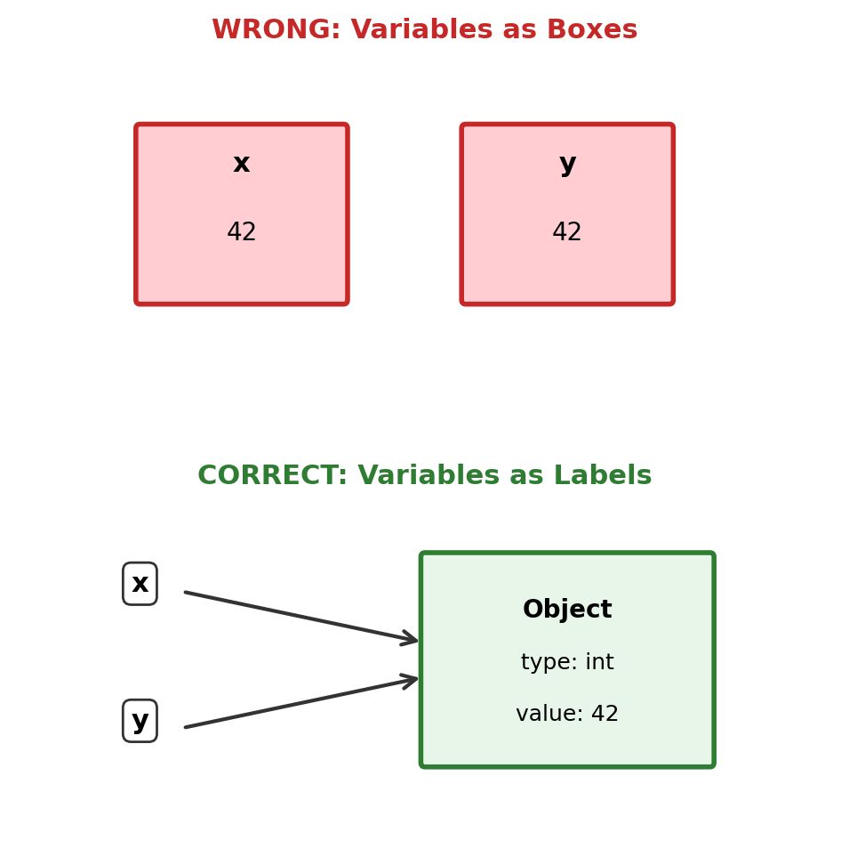
Immutable types (int, str, tuple): cannot be modified in place—operations create new objects.
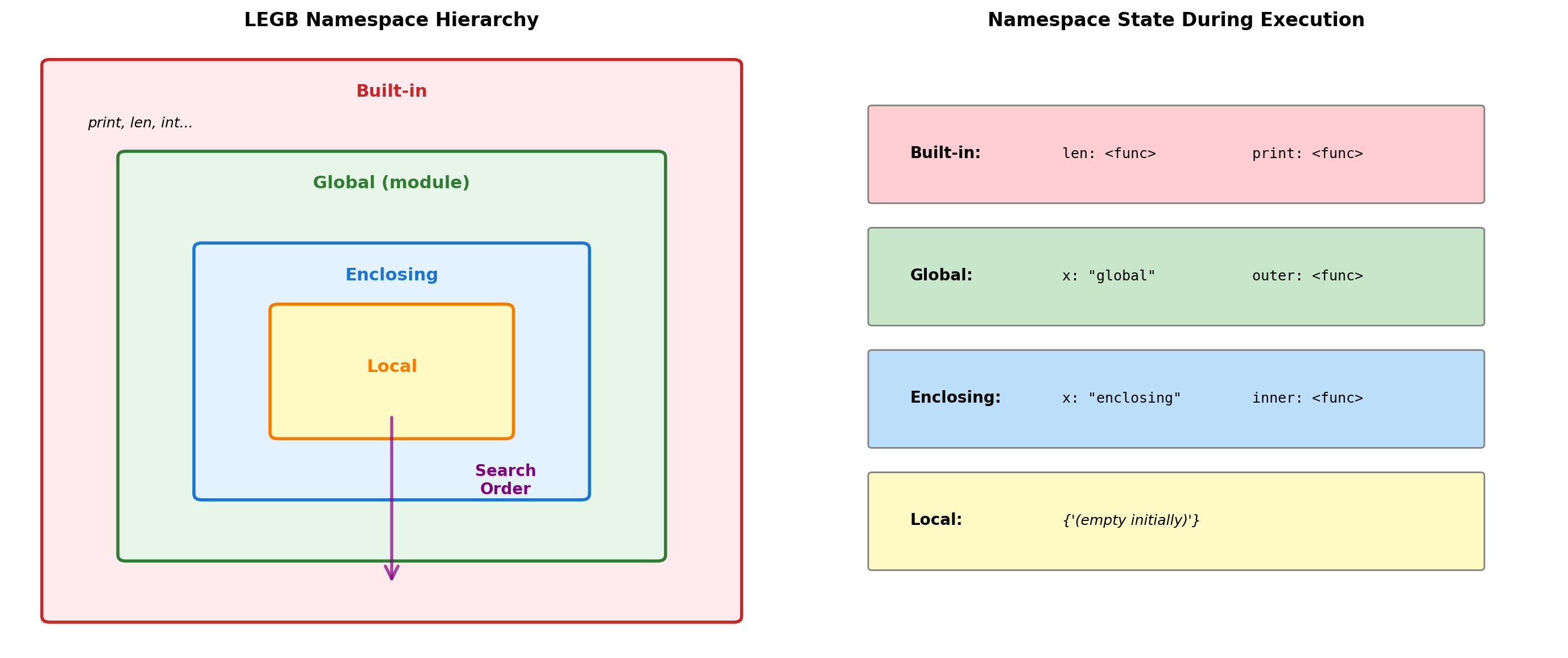
Namespace Resolution: The LEGB Rule
Python resolves names through a hierarchy of namespace dictionaries.
x = "global"  # Global namespace

def outer():
    x = "enclosing"  # Enclosing namespace

    def inner():
        print(f"Reading x: {x}")  # LEGB search finds enclosing

    def inner_local():
        x = "local"  # Creates local binding
        print(f"Local x: {x}")

    inner()
    inner_local()
    print(f"Enclosing x: {x}")

outer()
print(f"Global x: {x}")

# Namespace modification
def show_namespace_dict():
    local_var = 42
    print(f"locals(): {locals()}")
    print(f"'local_var' in locals(): {'local_var' in locals()}")

show_namespace_dict()
Reading x: enclosing
Local x: local
Enclosing x: enclosing
Global x: global
locals(): {'local_var': 42}
'local_var' in locals(): TrueResolution Rules:
- Local: Current function’s namespace
- Enclosing: Outer function(s) namespace
- Global: Module-level namespace
- Built-in: Pre-defined names
Binding Behavior:
- Assignment creates local binding by default
globalkeyword binds to global namespacenonlocalbinds to enclosing namespace- Reading doesn’t create binding
# UnboundLocalError example
count = 0
def increment():
# Python sees assignment, creates local slot
# But referenced before assignment
try:
count += 1 # UnboundLocalError
except UnboundLocalError as e:
print(f"Error: {e}")
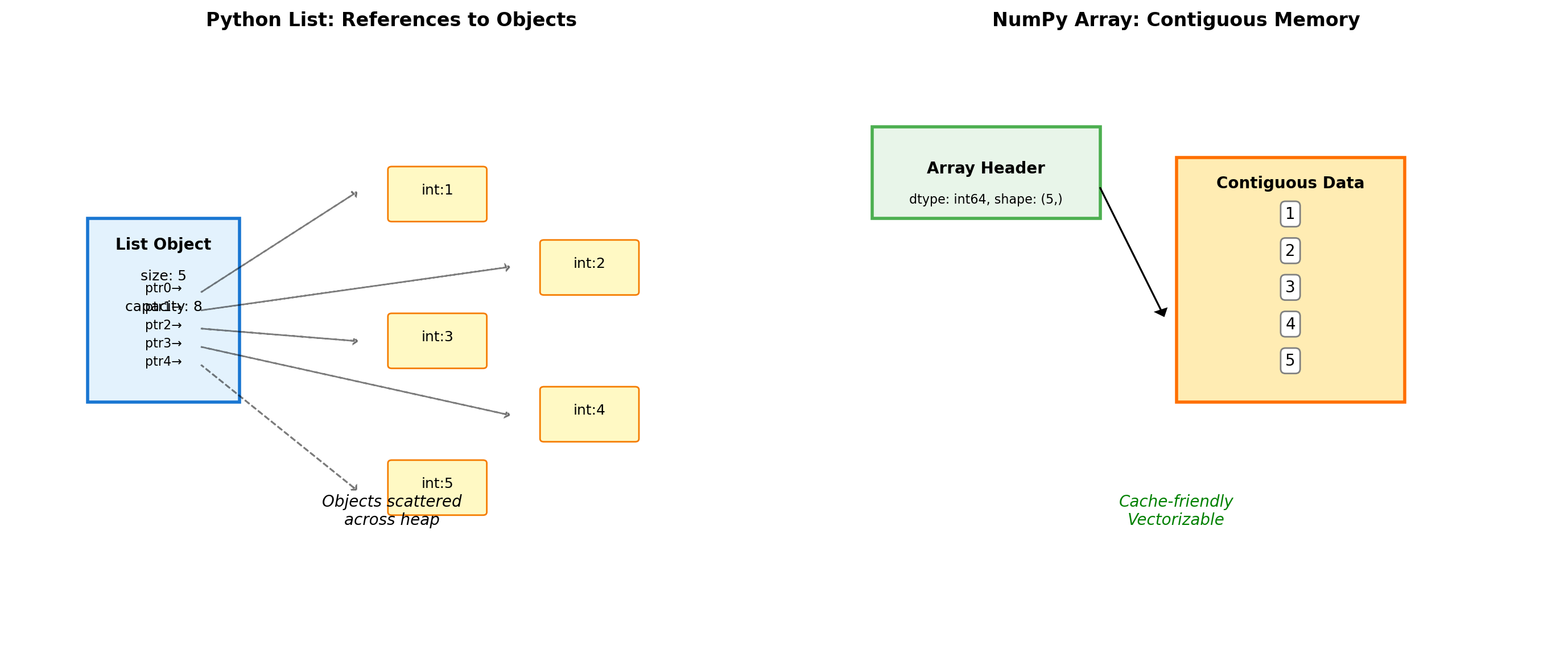
increment()Error: cannot access local variable 'count' where it is not associated with a valueLists vs Arrays: Memory Layout Matters
Python lists and NumPy arrays have different memory layouts.
import numpy as np

# Memory comparison
py_list = [1, 2, 3, 4, 5]
np_array = np.array([1, 2, 3, 4, 5])

print(f"Python list overhead: {sys.getsizeof(py_list)} bytes")
print(f"NumPy array overhead: {sys.getsizeof(np_array)} bytes")
print(f"NumPy data buffer: {np_array.nbytes} bytes")

# Performance impact
import timeit
lst = list(range(1000))
arr = np.arange(1000)

t_list = timeit.timeit(lambda: sum(lst), number=10000)
t_numpy = timeit.timeit(lambda: arr.sum(), number=10000)

print(f"\nSum 1000 elements:")
print(f"Python list: {t_list:.4f}s")
print(f"NumPy array: {t_numpy:.4f}s ({t_list/t_numpy:.1f}x faster)")
Python list overhead: 104 bytes
NumPy array overhead: 152 bytes
NumPy data buffer: 40 bytes
Sum 1000 elements:
Python list: 0.0242s
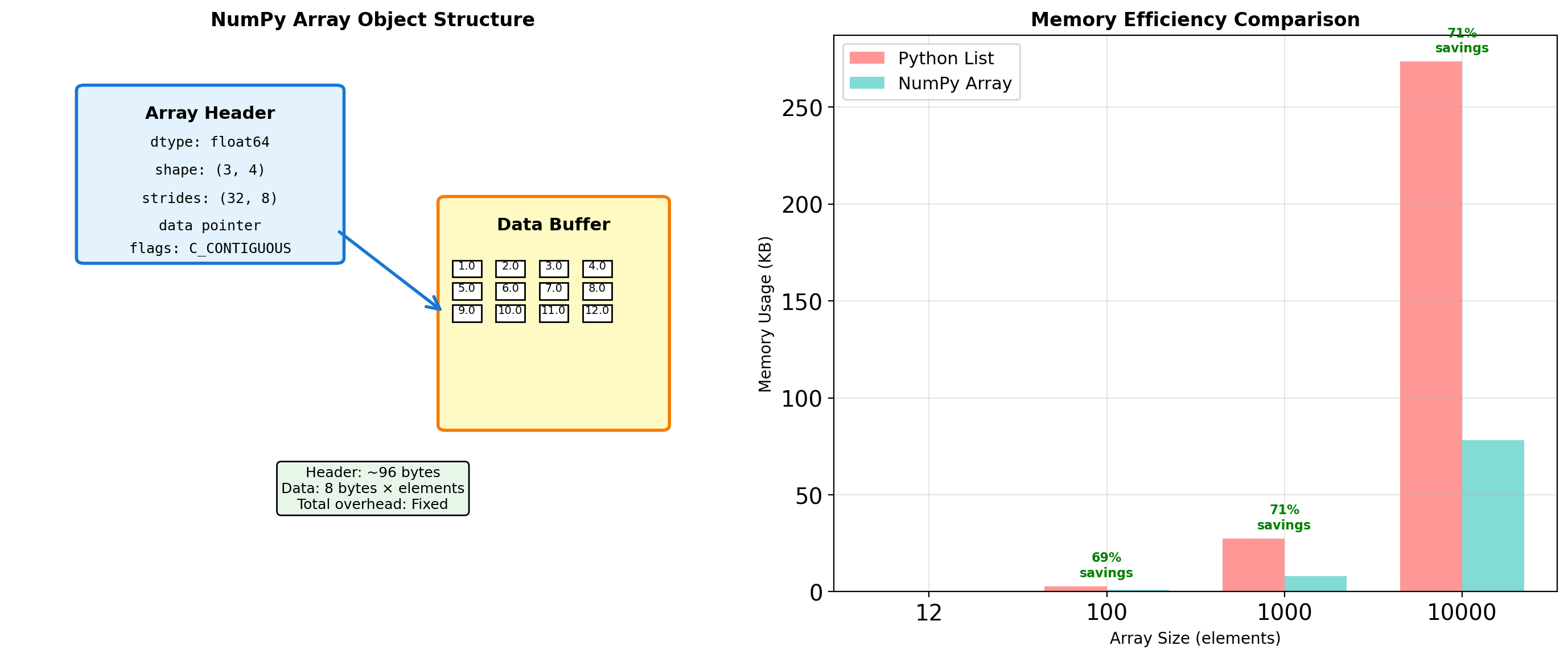
NumPy array: 0.0053s (4.6x faster)List cost per element:
- 8-byte pointer
- 28-byte int object
- ~36 bytes total per int
NumPy cost:
- ~100-byte header (fixed)
- 8 bytes per element (data only)
Why NumPy wins:
- No pointer chasing
- No per-element type checks
- Single C loop over contiguous memory
- Gap grows with array size
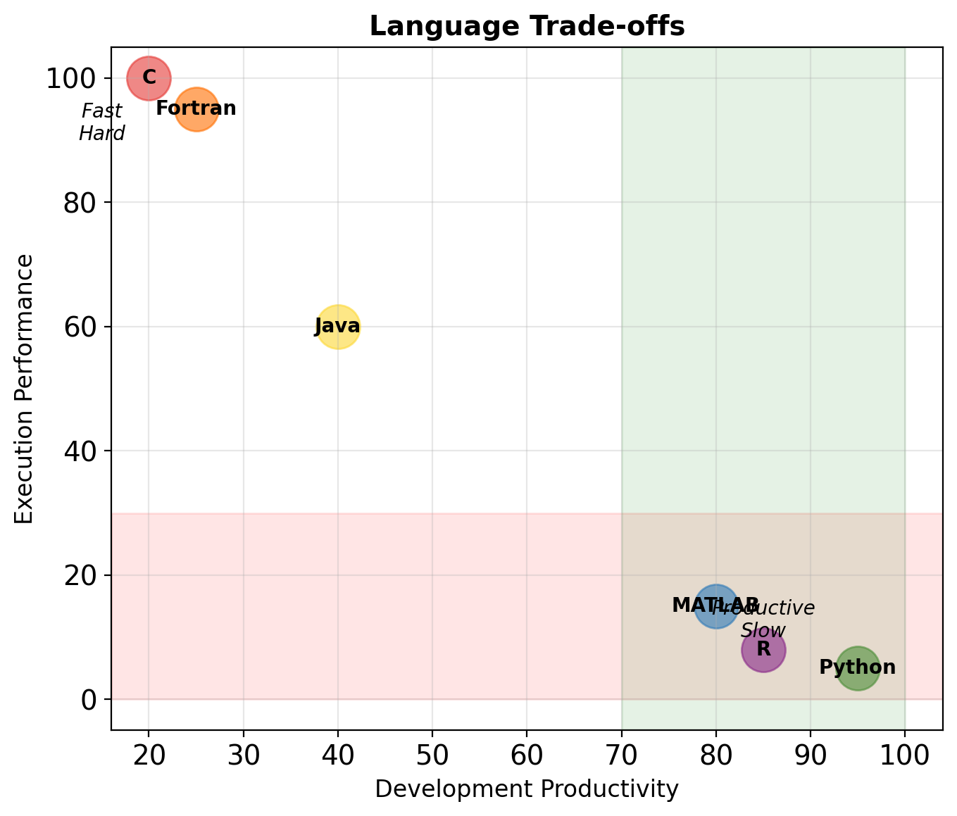
Python’s Execution Model
Why this matters:
- No separate compile step — edit and run immediately
- Runtime errors only — syntax errors found when line executes
- Slower than native code — bytecode interpretation has overhead
- Dynamic features — can modify code at runtime (
eval,exec)
Comparison:
| C++ | Java | Python | |
|---|---|---|---|
| Compile to | Machine code | JVM bytecode | PVM bytecode |
| Type checking | Compile time | Compile time | Runtime |
| Speed | Fast | Medium | Slow |
| Edit-run cycle | Slow | Medium | Fast |
Indexing and Slicing
Zero-based indexing. Negative indices count from the end. Slicing creates copies.
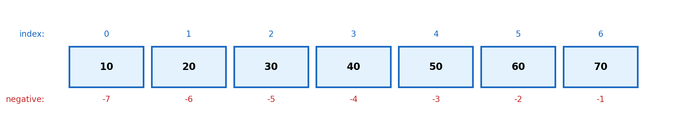
Slice syntax: [start:stop:step]
start: First index (inclusive), default 0stop: Last index (exclusive), default lenstep: Increment, default 1
data = [10, 20, 30, 40, 50, 60, 70]

print(f"data[2:5]  = {data[2:5]}")   # [30, 40, 50]
print(f"data[:3]   = {data[:3]}")    # [10, 20, 30]
print(f"data[4:]   = {data[4:]}")    # [50, 60, 70]
print(f"data[::2]  = {data[::2]}")   # [10, 30, 50, 70]
print(f"data[::-1] = {data[::-1]}")  # Reversed
print(f"data[1:-1] = {data[1:-1]}")  # [20, 30, 40, 50, 60]
data[2:5] = [30, 40, 50]
data[:3] = [10, 20, 30]
data[4:] = [50, 60, 70]
data[::2] = [10, 30, 50, 70]
data[::-1] = [70, 60, 50, 40, 30, 20, 10]
data[1:-1] = [20, 30, 40, 50, 60]Slicing creates copies (for lists):
original = [1, 2, 3, 4, 5]
copy = original[:]       # Shallow copy
copy[0] = 999
print(f"Original: {original}")
print(f"Copy: {copy}")
Original: [1, 2, 3, 4, 5]
Copy: [999, 2, 3, 4, 5]Slice assignment (modifies in place):
data = [1, 2, 3, 4, 5]
data[1:4] = [20, 30]     # Replace slice
print(f"After: {data}")

data[2:2] = [100, 200]   # Insert at index 2
print(f"After insert: {data}")
After: [1, 20, 30, 5]
After insert: [1, 20, 100, 200, 30, 5]Warning: NumPy arrays behave differently — slices are views, not copies.
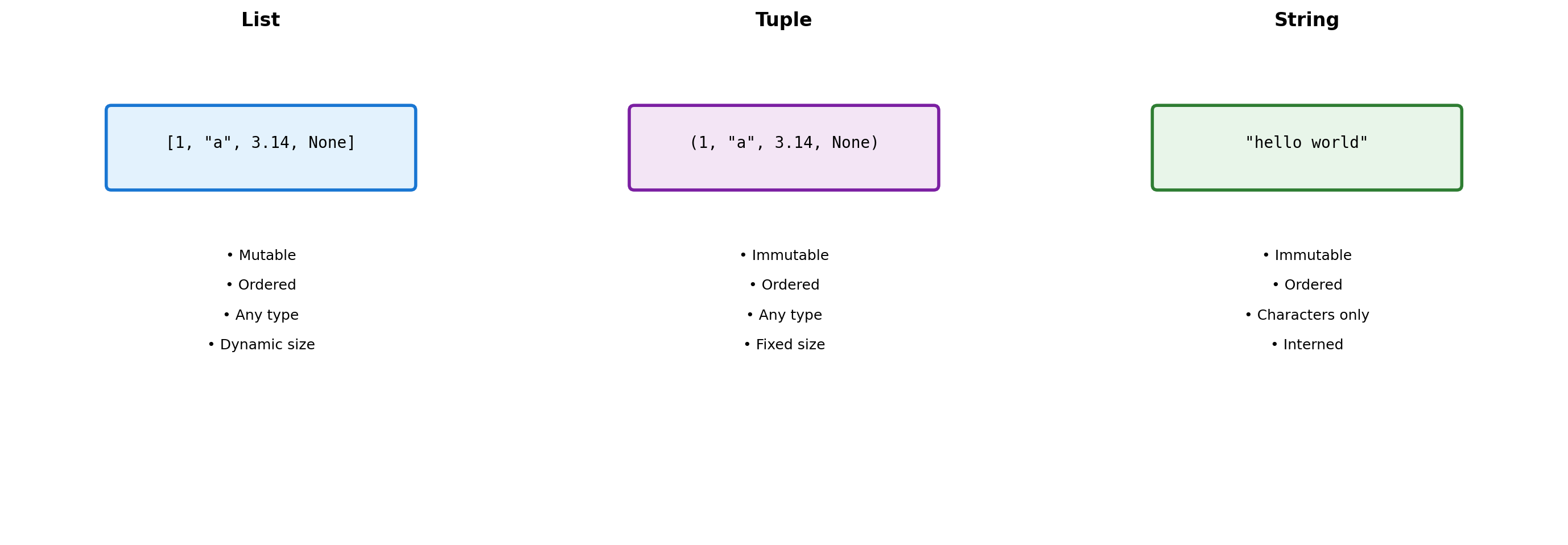
Sequence Types: Three Design Choices
Python provides three sequence types with different trade-offs.

Design Consequences:
- Lists allow heterogeneous data but pay indirection cost
- Tuples trade mutability for hashability and memory efficiency
- Strings optimize for text with specialized methods
import sys

# Memory comparison
lst = [1, 2, 3, 4, 5]
tup = (1, 2, 3, 4, 5)
string = "12345"

print("Memory usage:")
print(f"  List:   {sys.getsizeof(lst)} bytes")
print(f"  Tuple:  {sys.getsizeof(tup)} bytes")
print(f"  String: {sys.getsizeof(string)} bytes")

# Hashability determines dict key eligibility
print("\nCan be dict key:")
for obj, name in [(lst, 'List'), (tup, 'Tuple'), (string, 'String')]:
    try:
        d = {obj: 'value'}
        print(f"  {name}: Yes")
    except TypeError:
        print(f"  {name}: No")
Memory usage:
List: 104 bytes
Tuple: 80 bytes
String: 46 bytes
Can be dict key:
List: No
Tuple: Yes
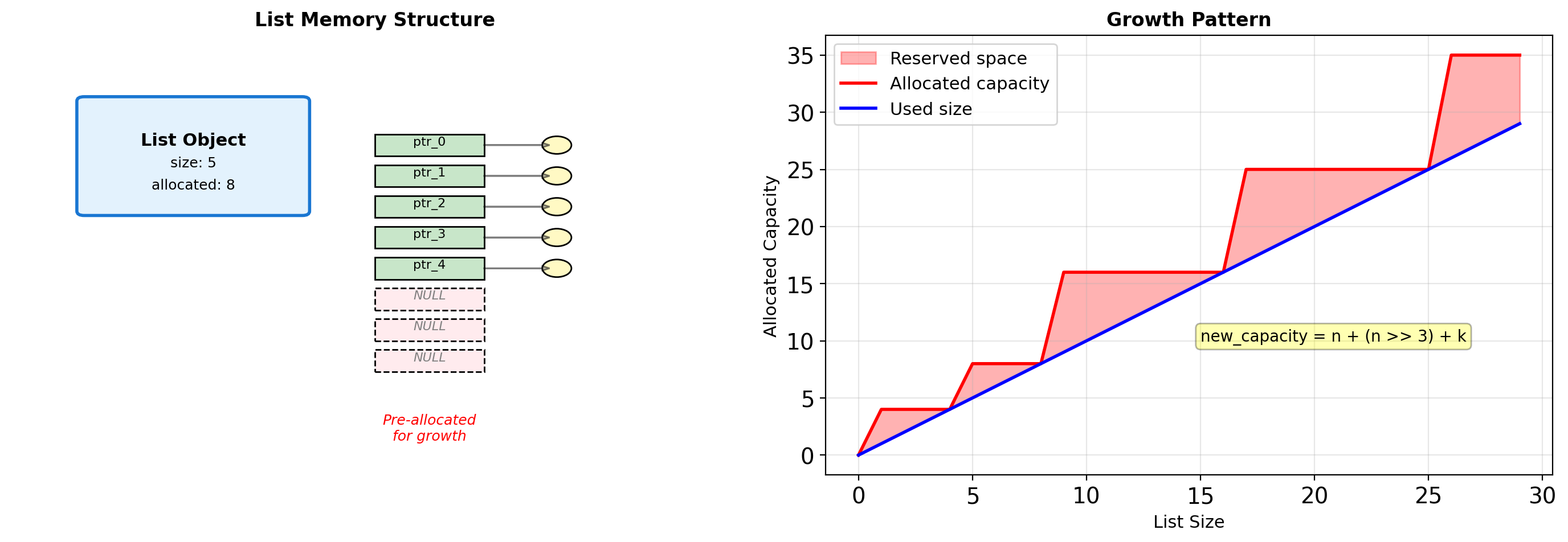
String: YesList Internals: Over-allocation Strategy
Lists allocate extra space to amortize the cost of growth.
# Observe allocation behavior
import sys

lst = []
sizes_and_caps = []

for i in range(20):
    lst.append(i)
    # Size includes list object overhead
    total_size = sys.getsizeof(lst)
    # Approximate capacity from size
    capacity = (total_size - sys.getsizeof([])) // 8
    sizes_and_caps.append((len(lst), capacity))

# Show growth points
print("Size → Capacity:")
last_cap = 0
for size, cap in sizes_and_caps:
    if cap != last_cap:
        print(f"  {size:2d} → {cap:2d} (grew by {cap - last_cap})")
        last_cap = cap
Size → Capacity:
1 → 4 (grew by 4)
5 → 8 (grew by 4)
9 → 16 (grew by 8)
17 → 24 (grew by 8)Growth Strategy:
When a list exceeds capacity, Python:
- Calculates new capacity using formula
- Allocates new pointer array
- Copies all existing pointers
- Frees old array
Cost Analysis:
- Append is O(1) amortized
- Individual append can trigger O(n) reallocation
- Trade memory for performance
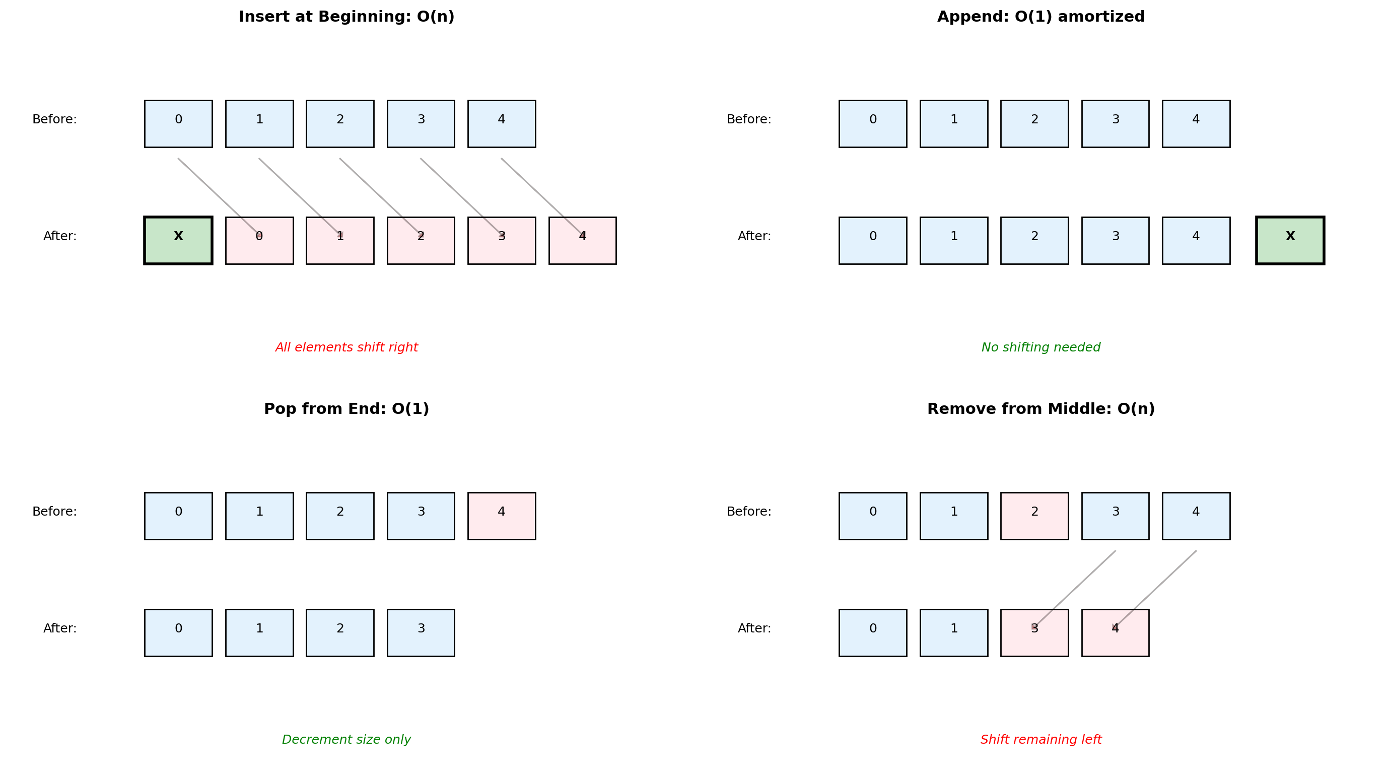
List Operations: Implementation Details
Different operations have different costs based on internal structure.
# Demonstrating operation costs
import time

def measure_operation(lst, operation, description):
    """Measure single operation time."""
    start = time.perf_counter()
    operation(lst)
    elapsed = time.perf_counter() - start
    return elapsed * 1e6  # Convert to microseconds

# Large list for measurable times
n = 100000
test_list = list(range(n))

# Operations
times = {}
times['append'] = measure_operation(test_list.copy(),
                                   lambda l: l.append(999),
                                   "Append")
times['insert_0'] = measure_operation(test_list.copy(),
                                      lambda l: l.insert(0, 999),
                                      "Insert at 0")
times['pop'] = measure_operation(test_list.copy(),
                                lambda l: l.pop(),
                                "Pop from end")
times['pop_0'] = measure_operation(test_list.copy(),
                                   lambda l: l.pop(0),
                                   "Pop from start")

print(f"Operation times (n={n}):")
for op, time in times.items():
    print(f"  {op:12s}: {time:8.2f} μs")
Operation times (n=100000):
append : 1.88 μs
insert_0 : 16.00 μs
pop : 0.21 μs
pop_0 : 12.96 μsDictionary Architecture: Open Addressing Hash Table
Dictionaries use open addressing with random probing for collision resolution.
# Dictionary internals
d = {'a': 1, 'b': 2, 'c': 3}

# Show hash values
for key in d:
    print(f"hash('{key}') = {hash(key):20d}")

# Dictionary growth
import sys
sizes = []
for i in range(20):
    d = {str(j): j for j in range(i)}
    sizes.append((i, sys.getsizeof(d)))

print("\nDict size growth:")
last_size = 0
for n, size in sizes:
    if size != last_size:
        print(f"  {n:2d} items: {size:4d} bytes")
        last_size = size
hash('a') = 1045829229493496788
hash('b') = -6016873841037565015
hash('c') = -969680730762518967
Dict size growth:
0 items: 64 bytes
1 items: 184 bytes
6 items: 272 bytes
11 items: 464 bytesDesign Choices:
- Open addressing: No separate chains, better cache locality
- 2/3 load factor: Resize when 2/3 full
- Perturbed probing: Reduces clustering
- Cached hash values: Store hash with key to avoid recomputation
Consequences:
- O(1) average case for all operations
- Order preserved since Python 3.7
- More memory than theoretical minimum
String Building: Algorithmic Complexity
Building strings efficiently requires understanding concatenation costs.
import io
import timeit

n = 1000
chunk = "x" * 10

# Method 1: Repeated concatenation (BAD)
def build_concat():
    s = ""
    for _ in range(n):
        s += chunk  # Creates new string each time
    return s

# Method 2: Join (GOOD)
def build_join():
    parts = []
    for _ in range(n):
        parts.append(chunk)
    return "".join(parts)

# Method 3: StringIO (GOOD)
def build_io():
    buffer = io.StringIO()
    for _ in range(n):
        buffer.write(chunk)
    return buffer.getvalue()

# Compare performance
t1 = timeit.timeit(build_concat, number=100)
t2 = timeit.timeit(build_join, number=100)
t3 = timeit.timeit(build_io, number=100)

print(f"Building {n}-chunk string (100 iterations):")
print(f"  Concatenation: {t1:.4f}s")
print(f"  Join:          {t2:.4f}s ({t1/t2:.1f}x faster)")
print(f"  StringIO:      {t3:.4f}s ({t1/t3:.1f}x faster)")
Building 1000-chunk string (100 iterations):
Concatenation: 0.0030s
Join: 0.0015s (2.0x faster)
StringIO: 0.0017s (1.8x faster)Collection Internals: Sets and Frozen Sets
Sets use the same hash table technology as dictionaries, optimized for membership testing.
# Set performance demonstration
import random

# Create test data
numbers = list(range(10000))
random.shuffle(numbers)

test_list = numbers[:5000]
test_set = set(test_list)

# Membership testing
lookups = random.sample(range(10000), 100)

import time

# List lookup
start = time.perf_counter()
for x in lookups:
    _ = x in test_list
list_time = time.perf_counter() - start

# Set lookup
start = time.perf_counter()
for x in lookups:
    _ = x in test_set
set_time = time.perf_counter() - start

print(f"100 lookups in collection of 5000:")
print(f"  List: {list_time*1000:.3f} ms")
print(f"  Set:  {set_time*1000:.3f} ms")
print(f"  Speedup: {list_time/set_time:.1f}x")

# Set operations
a = {1, 2, 3, 4, 5}
b = {4, 5, 6, 7, 8}

print(f"\nSet operations:")
print(f"  a & b = {a & b}")  # Intersection
print(f"  a | b = {a | b}")  # Union
print(f"  a - b = {a - b}")  # Difference
print(f"  a ^ b = {a ^ b}")  # Symmetric difference
100 lookups in collection of 5000:
List: 1.254 ms
Set: 0.034 ms
Speedup: 36.4x
Set operations:
a & b = {4, 5}
a | b = {1, 2, 3, 4, 5, 6, 7, 8}
a - b = {1, 2, 3}
a ^ b = {1, 2, 3, 6, 7, 8}Set Implementation:
- Same hash table as dict (no values)
- Average O(1) for add, remove, membership
- Set operations optimized with early termination
- Frozen sets are immutable and hashable
When to use sets:
- Membership testing in loops
- Removing duplicates
- Mathematical set operations
- When order doesn’t matter
Memory overhead:
- Minimum size: 8 slots
- Growth factor: 4x until 50k, then 2x
- ~30% more memory than list of same items
Shallow vs Deep Copying
Python’s default copying behavior can lead to unexpected aliasing.
import copy

# Create nested structure
original = [[1, 2], [3, 4], [5, 6]]

# Different copy methods
reference = original
shallow = original.copy()  # or list(original) or original[:]
deep = copy.deepcopy(original)

# Modify nested object
original[0].append(3)

print("After modifying original[0]:")
print(f"  original:  {original}")
print(f"  reference: {reference}")  # Changed
print(f"  shallow:   {shallow}")    # Changed!
print(f"  deep:      {deep}")       # Unchanged

# Identity checks
print("\nIdentity comparisons:")
print(f"  original is reference: {original is reference}")
print(f"  original is shallow:   {original is shallow}")
print(f"  original[0] is shallow[0]: {original[0] is shallow[0]}")  # True!
print(f"  original[0] is deep[0]:    {original[0] is deep[0]}")     # False
After modifying original[0]:
original: [[1, 2, 3], [3, 4], [5, 6]]
reference: [[1, 2, 3], [3, 4], [5, 6]]
shallow: [[1, 2, 3], [3, 4], [5, 6]]
deep: [[1, 2], [3, 4], [5, 6]]
Identity comparisons:
original is reference: True
original is shallow: False
original[0] is shallow[0]: True
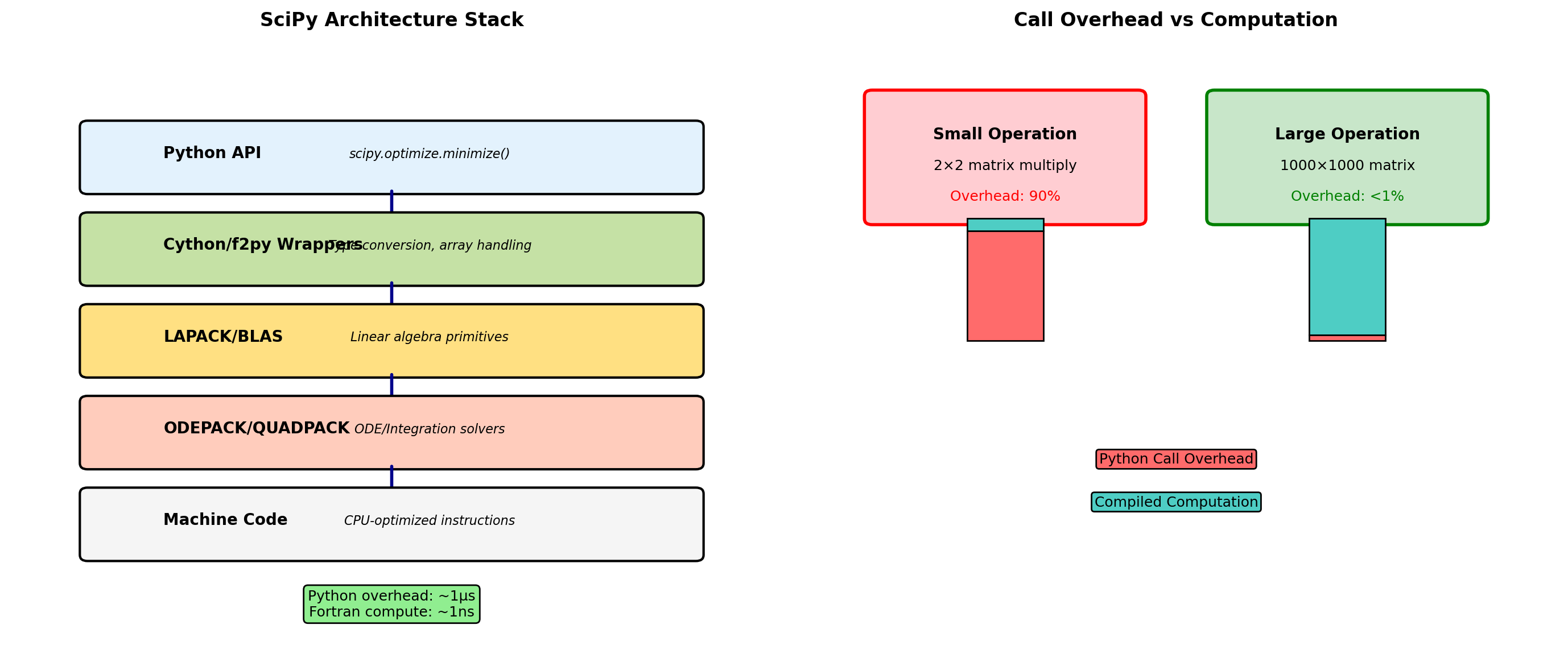
original[0] is deep[0]: FalseThe Python Scientific Stack
Python’s numerical libraries form a layered stack. Each layer builds on the ones below, trading some performance for convenience and expressiveness.
Each layer provides:
- Higher-level abstractions
- Automatic optimizations
- Platform independence
- Tested, maintained code
The goal: Write code at the highest appropriate level. Let NumPy/SciPy call optimized C/Fortran for you.
Example: Matrix multiply
# Don't write this
result = [[0]*n for _ in range(n)]
for i in range(n):
    for j in range(n):
        for k in range(n):
            result[i][j] += A[i][k] * B[k][j]

# Write this
result = A @ B  # Calls optimized BLAS
NumPy’s @ operator uses BLAS libraries that exploit CPU features (SIMD, cache blocking, parallelism).
Composition vs Inheritance
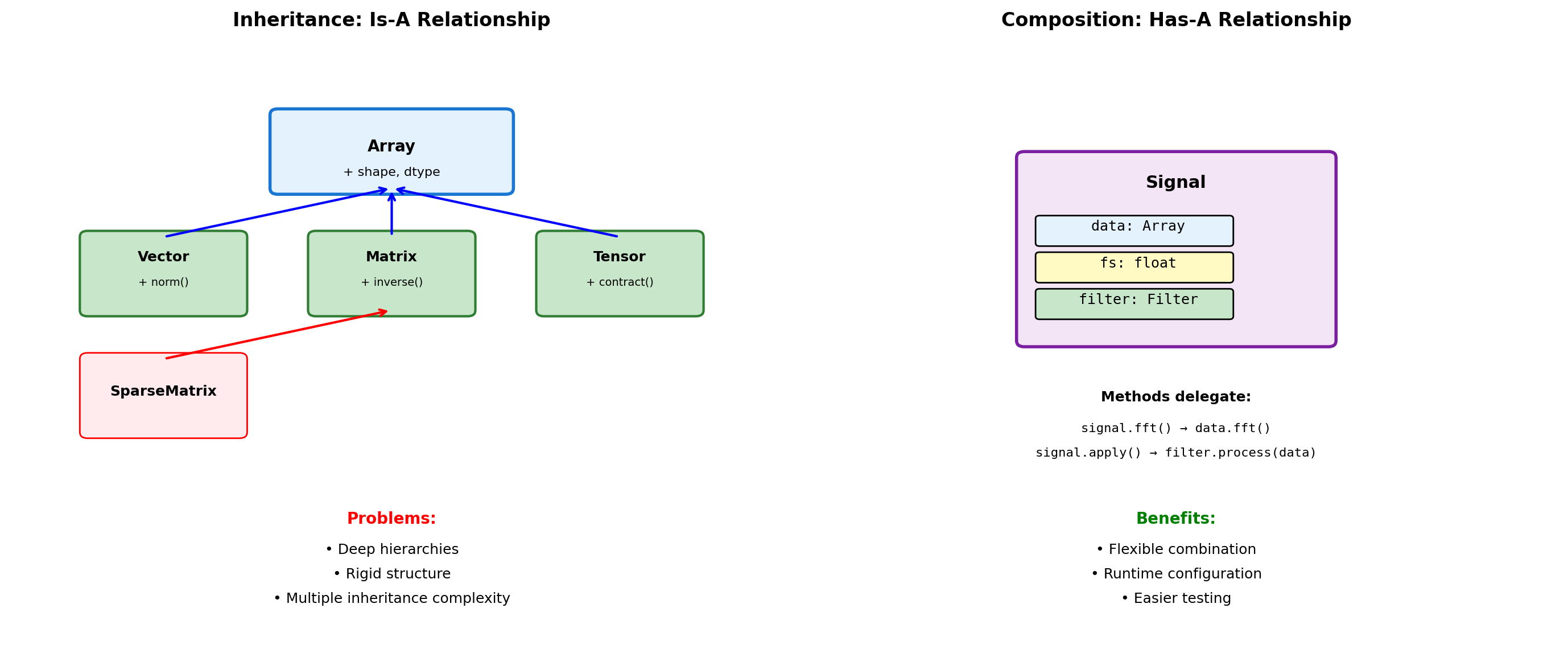
# Inheritance approach
class Vector(list):
    """Vector inherits from list."""

    def __init__(self, components):
        super().__init__(components)

    def magnitude(self):
        return sum(x**2 for x in self) ** 0.5

    def dot(self, other):
        return sum(a*b for a, b in zip(self, other))

# Problems with inheritance
v = Vector([3, 4])
print(f"Vector: {v}")
print(f"Magnitude: {v.magnitude()}")

# But inherits unwanted methods
v.reverse()  # Modifies in place!
print(f"After reverse: {v}")
v.append(5)  # Now 3D?
print(f"After append: {v}")
Vector: [3, 4]
Magnitude: 5.0
After reverse: [4, 3]
After append: [4, 3, 5]# Composition approach
class Signal:
"""Signal uses composition."""
def __init__(self, data, sample_rate):
self._data = np.array(data)
self.fs = sample_rate
self._filter = None
def __len__(self):
return len(self._data)
def __getitem__(self, idx):
return self._data[idx]
@property
def duration(self):
return len(self._data) / self.fs
def fft(self):
"""Delegate to NumPy."""
return np.fft.fft(self._data)
def resample(self, new_rate):
"""Return new Signal."""
ratio = new_rate / self.fs
new_length = int(len(self._data) * ratio)
new_data = np.interp(
np.linspace(0, len(self._data), new_length),
np.arange(len(self._data)),
self._data
)
return Signal(new_data, new_rate)
# Clean interface
sig = Signal([1, 2, 3, 4], sample_rate=100)
print(f"Duration: {sig.duration}s")
print(f"FFT shape: {sig.fft().shape}")Duration: 0.04s
FFT shape: (4,)Object Creation and Initialization
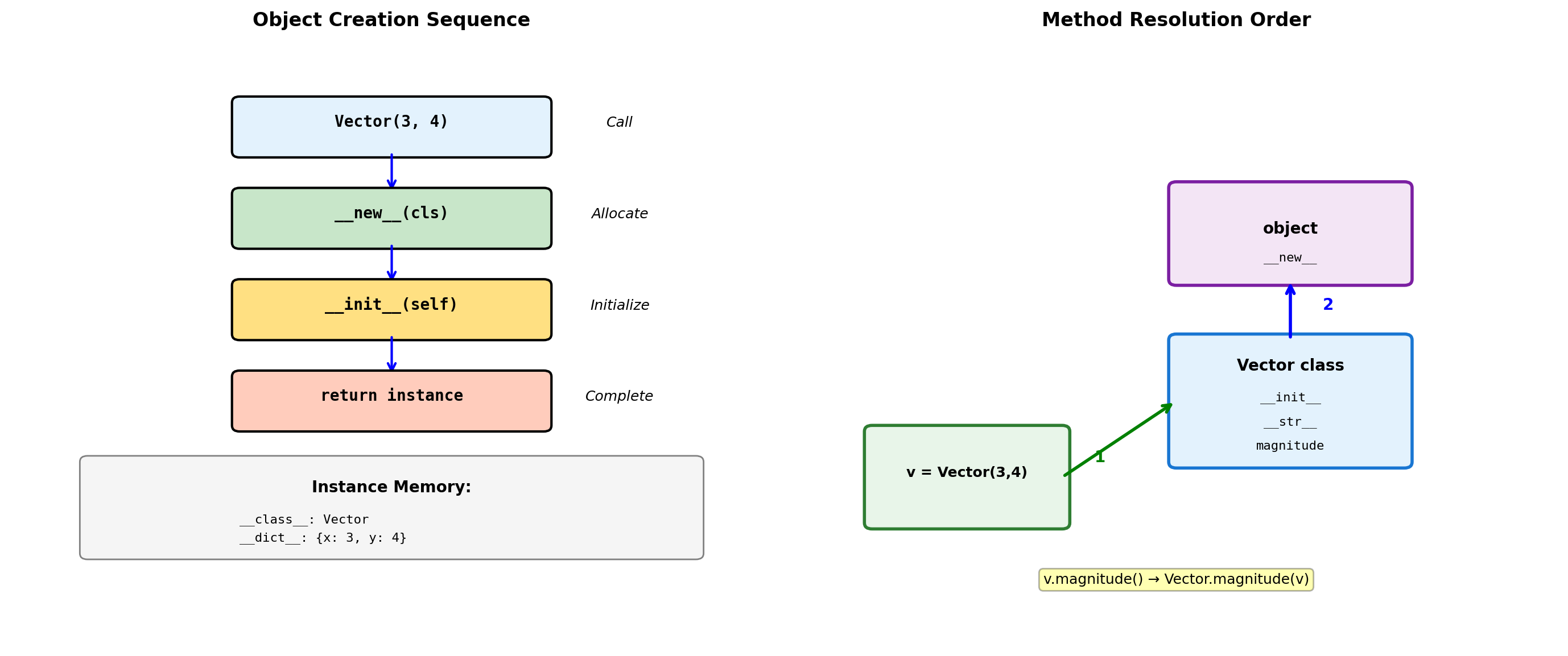
class Vector:
    """2D vector with special methods."""

    def __init__(self, x, y):
        """Initialize instance attributes."""
        self.x = x
        self.y = y

    def __repr__(self):
        """Developer representation (for debugging)."""
        return f"Vector({self.x}, {self.y})"

    def __str__(self):
        """User-friendly string representation."""
        return f"<{self.x}, {self.y}>"

    def magnitude(self):
        """Compute vector magnitude."""
        return (self.x**2 + self.y**2) ** 0.5

# Create instance
v = Vector(3, 4)

# Different string representations
print(f"repr(v): {repr(v)}")
print(f"str(v): {str(v)}")
print(f"Magnitude: {v.magnitude()}")

# Instance internals
print(f"\nInstance dict: {v.__dict__}")
print(f"Class: {v.__class__.__name__}")
repr(v): Vector(3, 4)
str(v): <3, 4>
Magnitude: 5.0
Instance dict: {'x': 3, 'y': 4}
Class: Vector# Method resolution demonstration
class Base:
def method(self):
return "Base"
def override_me(self):
return "Base version"
class Derived(Base):
def override_me(self):
return "Derived version"
def method(self):
# Call parent version
parent = super().method()
return f"{parent} → Derived"
d = Derived()
print(f"d.override_me(): {d.override_me()}")
print(f"d.method(): {d.method()}")
# MRO (Method Resolution Order)
print(f"\nMRO: {[cls.__name__ for cls in Derived.__mro__]}")
# Bound vs unbound methods
print(f"\nBound method: {d.method}")
print(f"Unbound: {Derived.method}")
print(f"Same function: {d.method.__func__ is Derived.method}")d.override_me(): Derived version
d.method(): Base → Derived
MRO: ['Derived', 'Base', 'object']
Bound method: <bound method Derived.method of <__main__.Derived object at 0x107e1b4d0>>
Unbound: <function Derived.method at 0x11fe23d80>
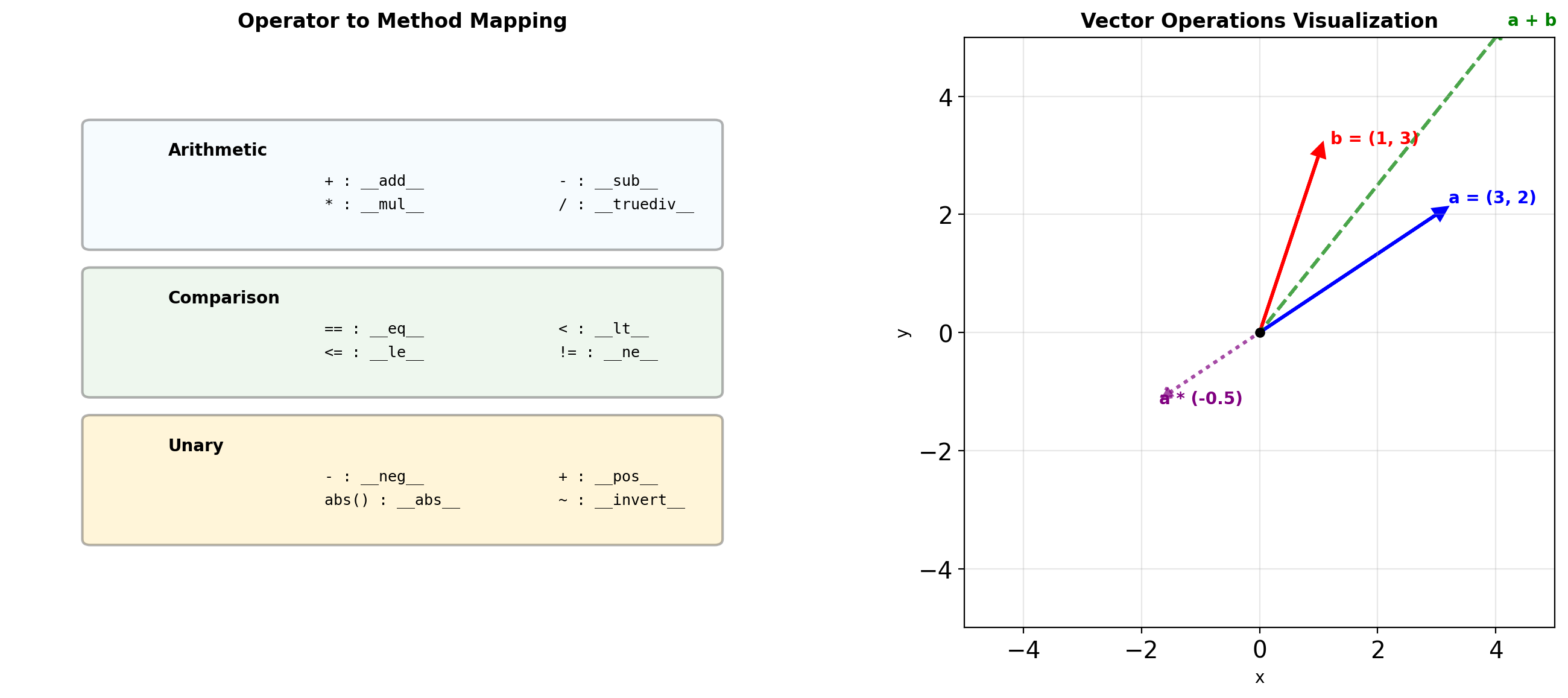
Same function: TrueOperator Overloading for Numerical Types
class Vector:
    def __init__(self, x, y):
        self.x = x
        self.y = y

    def __repr__(self):
        return f"Vector({self.x}, {self.y})"

    # Arithmetic operators
    def __add__(self, other):
        if isinstance(other, Vector):
            return Vector(self.x + other.x, self.y + other.y)
        return NotImplemented

    def __mul__(self, scalar):
        if isinstance(scalar, (int, float)):
            return Vector(self.x * scalar, self.y * scalar)
        return NotImplemented

    def __rmul__(self, scalar):
        """Right multiplication: scalar * vector"""
        return self.__mul__(scalar)

    def __neg__(self):
        return Vector(-self.x, -self.y)

    def __abs__(self):
        return (self.x**2 + self.y**2) ** 0.5

    # Comparison operators
    def __eq__(self, other):
        if not isinstance(other, Vector):
            return False
        return self.x == other.x and self.y == other.y

    def __lt__(self, other):
        """Compare by magnitude."""
        return abs(self) < abs(other)

# Usage
a = Vector(3, 4)
b = Vector(1, 2)

print(f"a = {a}")
print(f"b = {b}")
print(f"a + b = {a + b}")
print(f"2 * a = {2 * a}")
print(f"-a = {-a}")
print(f"|a| = {abs(a)}")
print(f"a == b: {a == b}")
print(f"a > b: {a > b}")
a = Vector(3, 4)
b = Vector(1, 2)
a + b = Vector(4, 6)
2 * a = Vector(6, 8)
-a = Vector(-3, -4)
|a| = 5.0
a == b: False
a > b: True# In-place operators
class Matrix:
def __init__(self, data):
self.data = np.array(data, dtype=float)
def __repr__(self):
return f"Matrix({self.data.tolist()})"
def __iadd__(self, other):
"""In-place addition: m += other"""
if isinstance(other, Matrix):
self.data += other.data
elif isinstance(other, (int, float)):
self.data += other
else:
return NotImplemented
return self # Must return self
def __matmul__(self, other):
"""Matrix multiplication: m @ other"""
if isinstance(other, Matrix):
return Matrix(self.data @ other.data)
return NotImplemented
def __getitem__(self, key):
"""Indexing: m[i, j]"""
return self.data[key]
def __setitem__(self, key, value):
"""Assignment: m[i, j] = value"""
self.data[key] = value
# Usage
m1 = Matrix([[1, 2], [3, 4]])
m2 = Matrix([[5, 6], [7, 8]])
print(f"m1 = {m1}")
print(f"m2 = {m2}")
print(f"m1 @ m2 = {m1 @ m2}")
print(f"m1[0, 1] = {m1[0, 1]}")
m1 += 10
print(f"After m1 += 10: {m1}")m1 = Matrix([[1.0, 2.0], [3.0, 4.0]])
m2 = Matrix([[5.0, 6.0], [7.0, 8.0]])
m1 @ m2 = Matrix([[19.0, 22.0], [43.0, 50.0]])
m1[0, 1] = 2.0
After m1 += 10: Matrix([[11.0, 12.0], [13.0, 14.0]])Properties and Descriptors

class Temperature:
    """Temperature with Celsius/Fahrenheit properties."""

    def __init__(self, celsius=0):
        self._celsius = celsius

    @property
    def celsius(self):
        """Getter for Celsius."""
        return self._celsius

    @celsius.setter
    def celsius(self, value):
        """Setter with validation."""
        if value < -273.15:
            raise ValueError(f"Temperature below absolute zero")
        self._celsius = value

    @property
    def fahrenheit(self):
        """Computed Fahrenheit property."""
        return self._celsius * 9/5 + 32

    @fahrenheit.setter
    def fahrenheit(self, value):
        """Set via Fahrenheit."""
        self.celsius = (value - 32) * 5/9

    @property
    def kelvin(self):
        """Read-only Kelvin property."""
        return self._celsius + 273.15

# Usage
temp = Temperature(25)
print(f"Celsius: {temp.celsius}°C")
print(f"Fahrenheit: {temp.fahrenheit}°F")
print(f"Kelvin: {temp.kelvin}K")

temp.fahrenheit = 86
print(f"\nAfter setting 86°F:")
print(f"Celsius: {temp.celsius}°C")

try:
    temp.celsius = -300
except ValueError as e:
    print(f"\nValidation error: {e}")
Celsius: 25°C
Fahrenheit: 77.0°F
Kelvin: 298.15K
After setting 86°F:
Celsius: 30.0°C
Validation error: Temperature below absolute zeroWhen to use properties:
- Computed values derived from other attributes
- Validation on attribute assignment
- Converting between representations (e.g., Celsius/Fahrenheit)
- Read-only attributes that shouldn’t be modified
Property mechanics:
- Getter: Called on
obj.attraccess - Setter: Called on
obj.attr = valueassignment - Deleter: Called on
del obj.attr - Properties are descriptors under the hood
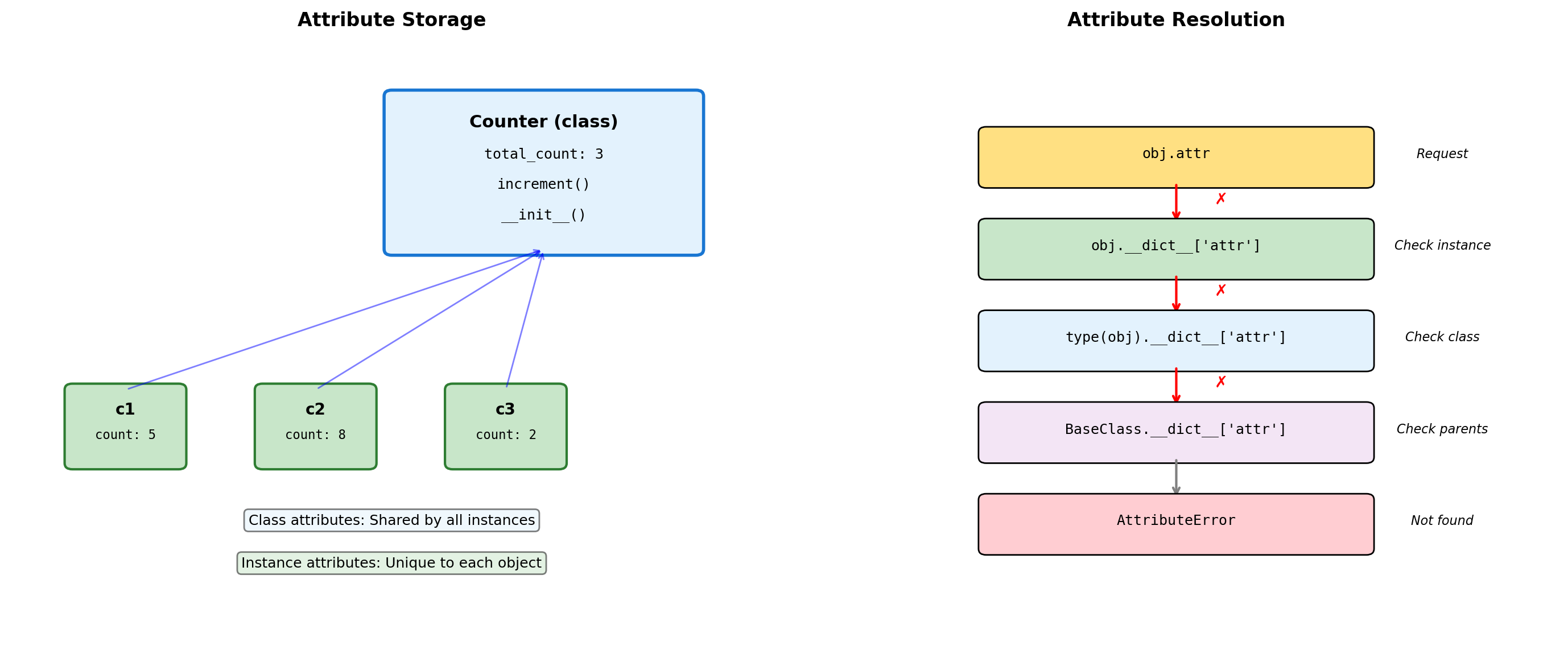
Class vs Instance Attributes
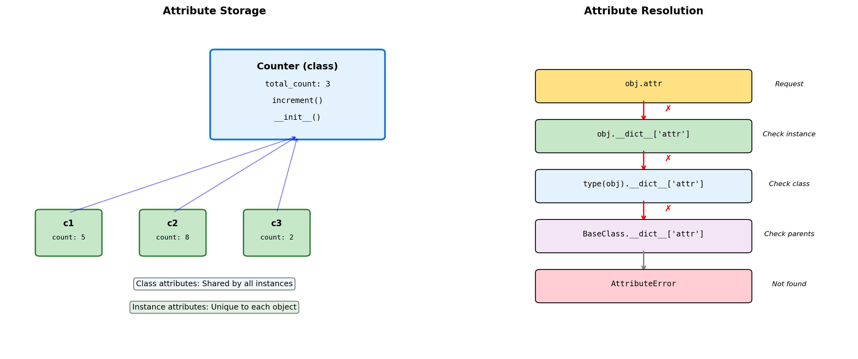
class Counter:
    """Demonstrates class vs instance attributes."""

    # Class attribute (shared)
    total_instances = 0
    default_step = 1

    def __init__(self, initial=0):
        # Instance attributes (unique)
        self.count = initial
        Counter.total_instances += 1

    def increment(self, step=None):
        # Use class default if not specified
        if step is None:
            step = self.default_step
        self.count += step

    @classmethod
    def get_total(cls):
        """Class method accesses class attributes."""
        return cls.total_instances

    @staticmethod
    def validate_step(step):
        """Static method - no access to instance or class."""
        return step > 0

# Create instances
c1 = Counter()
c2 = Counter(10)
c3 = Counter(20)

print(f"Total instances: {Counter.total_instances}")
print(f"c1.count: {c1.count}")
print(f"c2.count: {c2.count}")

# Modify class attribute
Counter.default_step = 5
c1.increment()
c2.increment()

print(f"\nAfter increment with step=5:")
print(f"c1.count: {c1.count}")
print(f"c2.count: {c2.count}")

# Instance shadows class attribute
c1.default_step = 10
print(f"\nc1.default_step: {c1.default_step}")
print(f"c2.default_step: {c2.default_step}")
Total instances: 3
c1.count: 0
c2.count: 10
After increment with step=5:
c1.count: 5
c2.count: 15
c1.default_step: 10
c2.default_step: 5Class vs instance attributes:
- Class attributes: Shared by all instances, defined at class level
- Instance attributes: Unique to each object, defined in
__init__ - Instance attributes shadow class attributes of the same name
Method types:
- Instance methods:
selfas first argument, access instance state - Class methods (
@classmethod):clsas first argument, access class state - Static methods (
@staticmethod): No implicit argument, utility functions
Common patterns:
- Class-level defaults modified per-instance
- Instance counters via class attributes
- Factory methods via
@classmethod
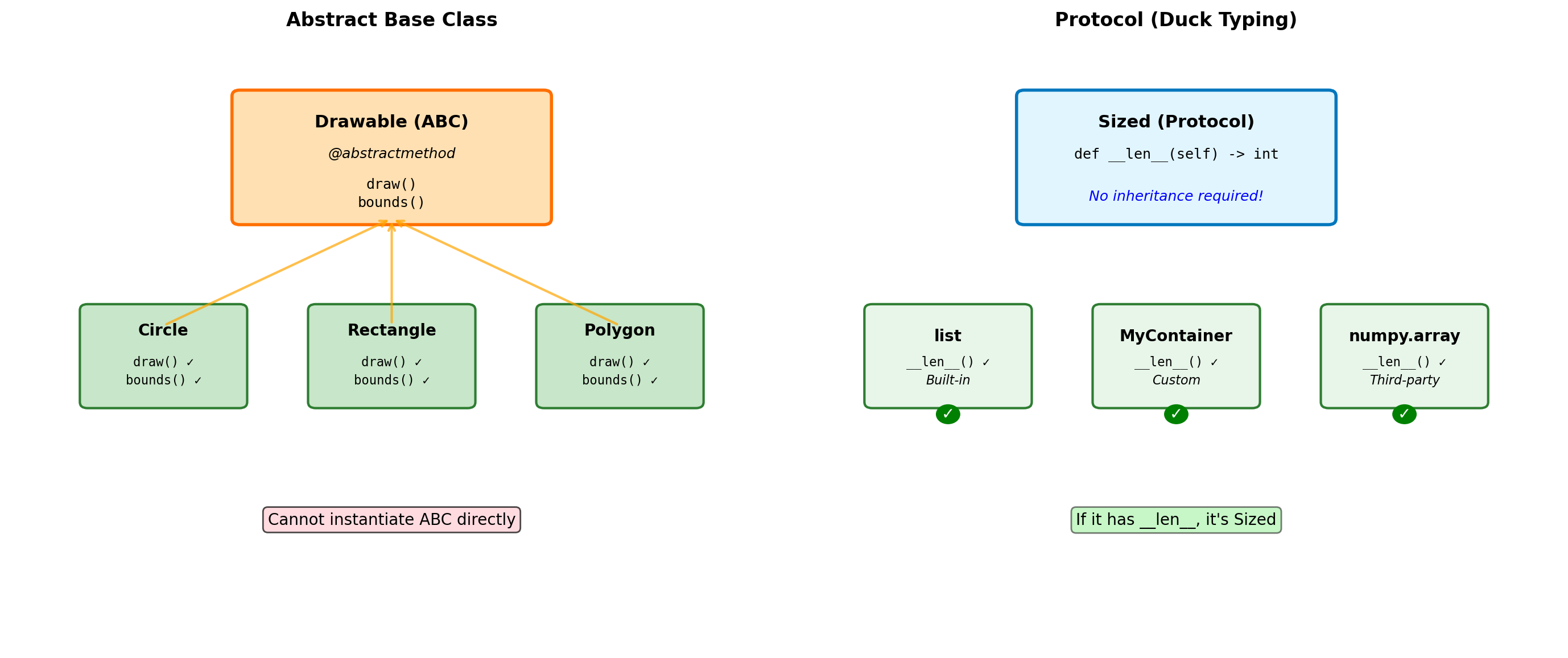
Abstract Base Classes and Protocols

from abc import ABC, abstractmethod
import math

class Shape(ABC):
    """Abstract base class for shapes."""

    @abstractmethod
    def area(self):
        """Must be implemented by subclasses."""
        pass

    @abstractmethod
    def perimeter(self):
        """Must be implemented by subclasses."""
        pass

    def describe(self):
        """Concrete method using abstract methods."""
        return f"Area: {self.area():.2f}, Perimeter: {self.perimeter():.2f}"

class Circle(Shape):
    def __init__(self, radius):
        self.radius = radius

    def area(self):
        return math.pi * self.radius ** 2

    def perimeter(self):
        return 2 * math.pi * self.radius

class Rectangle(Shape):
    def __init__(self, width, height):
        self.width = width
        self.height = height

    def area(self):
        return self.width * self.height

    def perimeter(self):
        return 2 * (self.width + self.height)

# Cannot instantiate ABC
try:
    shape = Shape()  # Error!
except TypeError as e:
    print(f"Error: {e}")

# Concrete classes work
circle = Circle(5)
rect = Rectangle(3, 4)

print(f"\nCircle: {circle.describe()}")
print(f"Rectangle: {rect.describe()}")

# Check inheritance
print(f"\nisinstance(circle, Shape): {isinstance(circle, Shape)}")
Error: Can't instantiate abstract class Shape without an implementation for abstract methods 'area', 'perimeter'
Circle: Area: 78.54, Perimeter: 31.42
Rectangle: Area: 12.00, Perimeter: 14.00
isinstance(circle, Shape): TrueWhen to use ABCs:
- Defining interfaces that must be implemented
- Template Method pattern (concrete methods calling abstract ones)
- Enforcing contracts in a class hierarchy
- When you want
isinstance()checks against the interface
ABC vs Duck Typing:
- ABCs: Explicit contracts, errors at instantiation time
- Duck typing: Implicit contracts, errors at call time
- Python prefers duck typing, but ABCs useful for frameworks
Built-in ABCs (collections.abc):
Iterable,Iterator,SequenceMapping,MutableMappingCallable,Hashable
Dataclasses for Numerical Structures
from dataclasses import dataclass, field
from typing import List
import numpy as np

@dataclass
class DataPoint:
    """Simple data container."""
    x: float
    y: float
    label: str = "unlabeled"
    metadata: dict = field(default_factory=dict)

    def distance_to(self, other):
        """Euclidean distance."""
        return ((self.x - other.x)**2 +
                (self.y - other.y)**2) ** 0.5

@dataclass(frozen=True)
class ImmutableVector:
    """Frozen dataclass - hashable."""
    x: float
    y: float
    z: float

    def magnitude(self):
        return (self.x**2 + self.y**2 + self.z**2) ** 0.5

    def __add__(self, other):
        """Return new vector (immutable)."""
        return ImmutableVector(
            self.x + other.x,
            self.y + other.y,
            self.z + other.z
        )

# Usage
p1 = DataPoint(3, 4)
p2 = DataPoint(6, 8, "target")

print(f"p1: {p1}")
print(f"p2: {p2}")
print(f"Distance: {p1.distance_to(p2):.2f}")

# Frozen vector
v1 = ImmutableVector(1, 2, 3)
v2 = ImmutableVector(4, 5, 6)
v3 = v1 + v2

print(f"\nv1 + v2 = {v3}")
print(f"Hashable: {hash(v1)}")

# Can use as dict key
vector_dict = {v1: "first", v2: "second"}
p1: DataPoint(x=3, y=4, label='unlabeled', metadata={})
p2: DataPoint(x=6, y=8, label='target', metadata={})
Distance: 5.00
v1 + v2 = ImmutableVector(x=5, y=7, z=9)
Hashable: 529344067295497451@dataclass(order=True)
class Measurement:
"""Sortable measurement with validation."""
timestamp: float = field(compare=True)
value: float = field(compare=False)
sensor_id: str = field(default="unknown", compare=False)
def __post_init__(self):
"""Validation after initialization."""
if self.value < 0:
raise ValueError(f"Negative value: {self.value}")
if self.timestamp < 0:
raise ValueError(f"Invalid timestamp: {self.timestamp}")
# Sorting by timestamp
measurements = [
Measurement(100.5, 23.4, "A1"),
Measurement(99.2, 25.1, "A2"),
Measurement(101.3, 22.8, "A1"),
]
sorted_measurements = sorted(measurements)
print("Sorted by timestamp:")
for m in sorted_measurements:
print(f" t={m.timestamp}: {m.value}")
# Performance comparison
from dataclasses import dataclass
import sys
@dataclass(slots=True)
class SlottedPoint:
x: float
y: float
@dataclass
class RegularPoint:
x: float
y: float
sp = SlottedPoint(1, 2)
rp = RegularPoint(1, 2)
print(f"\nMemory usage:")
print(f" With slots: {sys.getsizeof(sp)} bytes")
print(f" Regular: {sys.getsizeof(rp) + sys.getsizeof(rp.__dict__)} bytes")Sorted by timestamp:
t=99.2: 25.1
t=100.5: 23.4
t=101.3: 22.8
Memory usage:
With slots: 48 bytes
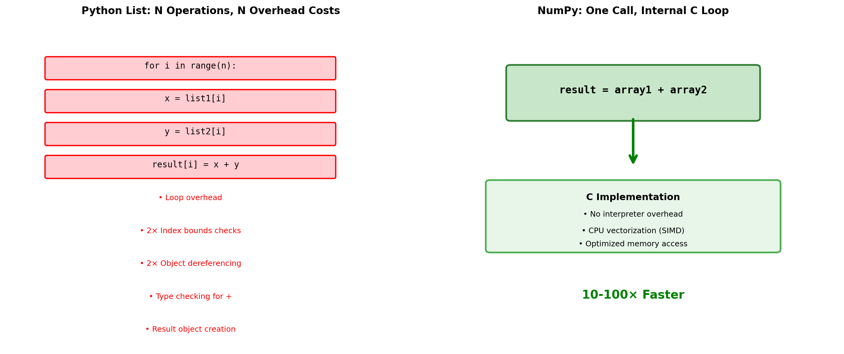
Regular: 344 bytesWhy NumPy Exists: Python’s Performance Wall
NumPy solves Python’s fundamental limitation: every operation triggers expensive interpreter overhead.

import numpy as np
import timeit

# Demonstrate the performance difference
def python_add(list1, list2):
    """Pure Python element-wise addition."""
    result = []
    for i in range(len(list1)):
        result.append(list1[i] + list2[i])
    return result

def numpy_add(arr1, arr2):
    """NumPy vectorized addition."""
    return arr1 + arr2

# Test data
size = 100000
py_list1 = list(range(size))
py_list2 = list(range(size, size*2))
np_arr1 = np.array(py_list1)
np_arr2 = np.array(py_list2)

# Benchmark
t_python = timeit.timeit(
    lambda: python_add(py_list1, py_list2),
    number=10
)
t_numpy = timeit.timeit(
    lambda: numpy_add(np_arr1, np_arr2),
    number=10
)

print(f"Adding {size:,} numbers (10 iterations):")
print(f"  Python lists: {t_python:.3f}s")
print(f"  NumPy arrays: {t_numpy:.3f}s")
print(f"  Speedup: {t_python/t_numpy:.0f}x")

# Show function call overhead
python_ops = size * 4  # loop, 2 indexes, 1 addition per iteration
numpy_ops = 1  # single function call
print(f"\nPython operations: {python_ops:,}")
print(f"NumPy operations: {numpy_ops}")
print(f"Overhead reduction: {python_ops/numpy_ops:.0f}x")
Adding 100,000 numbers (10 iterations):
Python lists: 0.024s
NumPy arrays: 0.000s
Speedup: 66x
Python operations: 400,000
NumPy operations: 1
Overhead reduction: 400000xThe NumPy Solution:
- Homogeneous data - All elements same type, enabling compact storage
- Contiguous memory - Cache-friendly access patterns
- Vectorized operations - Single Python call processes entire arrays
- C implementation - Inner loops run at machine speed
Cost of flexibility:
- Python lists can mix types, NumPy arrays cannot
- Dynamic resizing is expensive in NumPy
- Small arrays may be slower due to overhead
When NumPy wins:
- Numerical computations on large datasets
- Element-wise operations
- Mathematical functions (sin, cos, exp)
- Linear algebra operations
Array Object Internals: More Than Just Data
NumPy arrays separate metadata from data, enabling views and broadcasting without copying.
import numpy as np
import sys

# Examine array internals
arr = np.arange(12, dtype=np.float64).reshape(3, 4)

print("Array structure analysis:")
print(f"  Array object size: {sys.getsizeof(arr)} bytes")
print(f"  Data buffer size: {arr.nbytes} bytes")
print(f"  Shape: {arr.shape}")
print(f"  Strides: {arr.strides}")  # Bytes to next element in each dimension
print(f"  Data type: {arr.dtype}")
print(f"  Item size: {arr.itemsize} bytes")

# Memory layout inspection
print(f"\nMemory layout:")
print(f"  C-contiguous: {arr.flags['C_CONTIGUOUS']}")
print(f"  F-contiguous: {arr.flags['F_CONTIGUOUS']}")
print(f"  Owns data: {arr.flags['OWNDATA']}")

# Compare with Python list
py_list = arr.tolist()
print(f"\nMemory comparison for 12 elements:")
print(f"  NumPy array: {sys.getsizeof(arr) + arr.nbytes} bytes total")
print(f"  Python list: {sys.getsizeof(py_list)} bytes (list)")

# Calculate Python list element overhead
element_overhead = sum(sys.getsizeof(x) for row in py_list for x in row)
print(f"  Python objects: {element_overhead} bytes (elements)")
print(f"  Python total: {sys.getsizeof(py_list) + element_overhead} bytes")

# Show memory addressing
print(f"\nMemory addressing:")
print(f"  Base address: {arr.__array_interface__['data'][0]:#x}")
print(f"  Element [0,0] offset: 0 bytes")
print(f"  Element [0,1] offset: {arr.strides[1]} bytes")
print(f"  Element [1,0] offset: {arr.strides[0]} bytes")

# Demonstrate stride calculation
row, col = 1, 2
offset = row * arr.strides[0] + col * arr.strides[1]
print(f"  Element [1,2] offset: {offset} bytes → value {arr[1,2]}")
Array structure analysis:
Array object size: 128 bytes
Data buffer size: 96 bytes
Shape: (3, 4)
Strides: (32, 8)
Data type: float64
Item size: 8 bytes
Memory layout:
C-contiguous: True
F-contiguous: False
Owns data: False
Memory comparison for 12 elements:
NumPy array: 224 bytes total
Python list: 80 bytes (list)
Python objects: 288 bytes (elements)
Python total: 368 bytes
Memory addressing:
Base address: 0x11be4fa00
Element [0,0] offset: 0 bytes
Element [0,1] offset: 8 bytes
Element [1,0] offset: 32 bytes
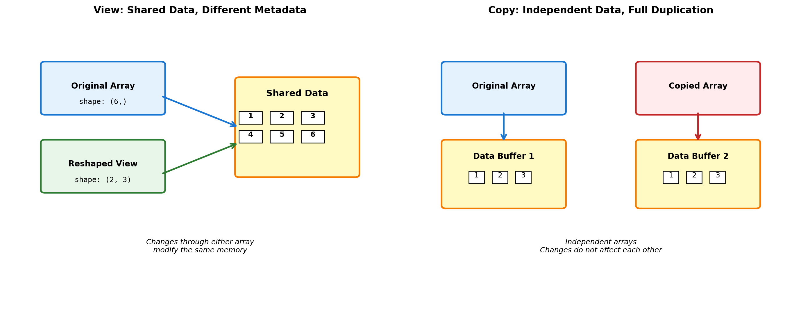
Element [1,2] offset: 48 bytes → value 6.0Array metadata enables:
- Reshaping without copying - Same data, different view
- Slicing creates views - No memory duplication
- Broadcasting - Operations on different-shaped arrays
- Memory mapping - Work with files larger than RAM
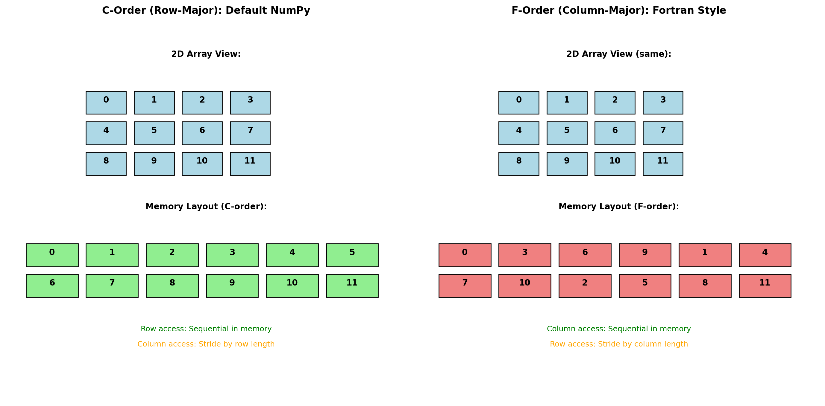
Memory Layout: Row-Major vs Column-Major
Array element ordering in memory affects performance significantly due to CPU cache behavior.
import numpy as np
import timeit

# Create arrays with different memory layouts
size = 1000
c_array = np.random.rand(size, size)  # C-order (default)
f_array = np.asfortranarray(c_array)  # F-order copy

print("Memory layout comparison:")
print(f"C-order shape: {c_array.shape}, strides: {c_array.strides}")
print(f"F-order shape: {f_array.shape}, strides: {f_array.strides}")
print(f"C-order flags: C={c_array.flags.c_contiguous}, F={c_array.flags.f_contiguous}")
print(f"F-order flags: C={f_array.flags.c_contiguous}, F={f_array.flags.f_contiguous}")

# Row access performance (C-order wins)
def sum_rows(arr):
    return [np.sum(arr[i, :]) for i in range(100)]

# Column access performance (F-order wins)
def sum_cols(arr):
    return [np.sum(arr[:, j]) for j in range(100)]

t_c_rows = timeit.timeit(lambda: sum_rows(c_array), number=100)
t_f_rows = timeit.timeit(lambda: sum_rows(f_array), number=100)

t_c_cols = timeit.timeit(lambda: sum_cols(c_array), number=100)
t_f_cols = timeit.timeit(lambda: sum_cols(f_array), number=100)

print(f"\nRow access performance (100 iterations):")
print(f"  C-order: {t_c_rows:.3f}s")
print(f"  F-order: {t_f_rows:.3f}s ({t_f_rows/t_c_rows:.1f}x slower)")

print(f"\nColumn access performance (100 iterations):")
print(f"  C-order: {t_c_cols:.3f}s")
print(f"  F-order: {t_f_cols:.3f}s ({t_c_cols/t_f_cols:.1f}x faster)")
Memory layout comparison:
C-order shape: (1000, 1000), strides: (8000, 8)
F-order shape: (1000, 1000), strides: (8, 8000)
C-order flags: C=True, F=False
F-order flags: C=False, F=True
Row access performance (100 iterations):
C-order: 0.011s
F-order: 0.014s (1.2x slower)
Column access performance (100 iterations):
C-order: 0.013s
F-order: 0.010s (1.2x faster)Memory layout matters because:
- CPU cache lines - Fetch 64-byte chunks from RAM
- Spatial locality - Adjacent memory access is faster
- Prefetching - CPU predicts sequential access patterns
C-order (row-major):
- Default in NumPy, C, Python
- Rows stored contiguously
- Better for row operations
F-order (column-major):
- Default in Fortran, MATLAB, R
- Columns stored contiguously
- Better for column operations
- Required by some BLAS routines
Performance implications:
- Cache misses can cause 100× slowdowns
- Matrix algorithms should match layout
- Transpose operations may change layout
Views vs Copies: Memory Management Semantics
NumPy operations can either create views (sharing data) or copies (duplicating data).
import numpy as np

# Create original array
original = np.arange(12).reshape(3, 4)
print("Original array:")
print(original)

# View operations (share data)
view_reshaped = original.reshape(4, 3)
view_slice = original[1:, :]
view_transpose = original.T

print(f"\nView operations (share data):")
print(f"  original.base is None: {original.base is None}")
print(f"  view_reshaped.base is original: {view_reshaped.base is original}")
print(f"  view_slice.base is original: {view_slice.base is original}")
print(f"  view_transpose.base is original: {view_transpose.base is original}")

# Test sharing - modify through view
original[0, 0] = 999
print(f"\nAfter setting original[0,0] = 999:")
print(f"  original[0,0] = {original[0,0]}")
print(f"  view_reshaped[0,0] = {view_reshaped[0,0]}")  # Same memory!

# Copy operations (independent data)
copy_array = original.copy()
copy_flatten = original.flatten()  # Unlike ravel(), always copies

print(f"\nCopy operations (independent data):")
print(f"  copy_array.base is None: {copy_array.base is None}")
print(f"  copy_flatten.base is None: {copy_flatten.base is None}")

# Test independence
original[1, 1] = 888
print(f"\nAfter setting original[1,1] = 888:")
print(f"  original[1,1] = {original[1,1]}")
print(f"  copy_array[1,1] = {copy_array[1,1]}")  # Independent!

# Memory usage comparison
import sys
print(f"\nMemory usage:")
print(f"  Original: {original.nbytes} bytes")
print(f"  View: {view_reshaped.nbytes} bytes data (shares with original)")
print(f"  Copy: {copy_array.nbytes} bytes (independent)")
print(f"  Total with view: ~{original.nbytes} bytes")
print(f"  Total with copy: ~{original.nbytes + copy_array.nbytes} bytes")

# Dangerous view scenario
def demonstrate_view_trap():
    """Common mistake with views."""
    data = np.arange(10)
    subset = data[::2]  # Every other element (view)

    # Modify original
    data.fill(0)

    return subset  # Returns modified data!

result = demonstrate_view_trap()
print(f"\nView trap result: {result}")  # All zeros, not original values!
Original array:
[[ 0 1 2 3]
[ 4 5 6 7]
[ 8 9 10 11]]
View operations (share data):
original.base is None: False
view_reshaped.base is original: False
view_slice.base is original: False
view_transpose.base is original: False
After setting original[0,0] = 999:
original[0,0] = 999
view_reshaped[0,0] = 999
Copy operations (independent data):
copy_array.base is None: True
copy_flatten.base is None: True
After setting original[1,1] = 888:
original[1,1] = 888
copy_array[1,1] = 5
Memory usage:
Original: 96 bytes
View: 96 bytes data (shares with original)
Copy: 96 bytes (independent)
Total with view: ~96 bytes
Total with copy: ~192 bytes
View trap result: [0 0 0 0 0]View operations (share data):
- Slicing:
arr[start:stop] - Reshaping:
arr.reshape() - Transposing:
arr.T - Index arrays with step:
arr[::2]
Copy operations (new data):
- Explicit copy:
arr.copy() - Fancy indexing:
arr[[1,3,5]] - Boolean indexing:
arr[arr > 0] - Some functions:
flatten(),ravel()(conditionally)
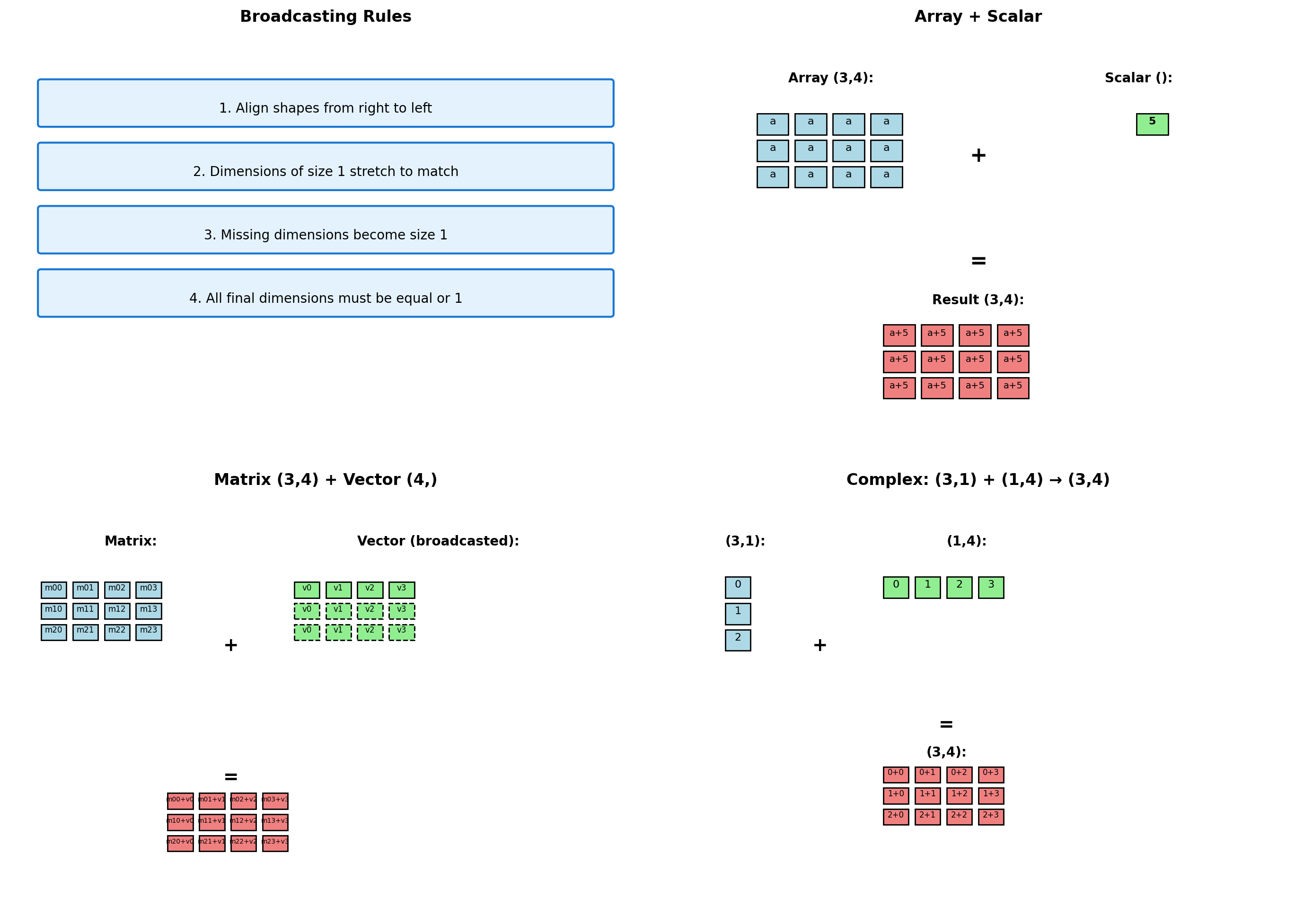
Broadcasting: Operations on Different-Shaped Arrays
Broadcasting enables operations between arrays of different shapes without explicit loops or memory duplication.
import numpy as np

# Broadcasting examples with shape analysis
def show_broadcast(a, b, operation_name):
    """Demonstrate broadcasting between two arrays."""
    print(f"\n{operation_name}:")
    print(f"  Array A shape: {a.shape}")

    # Handle scalar case
    if np.isscalar(b):
        print(f"  Array B: scalar ({b})")
        b_bytes = 8  # Approximate scalar size
    else:
        print(f"  Array B shape: {b.shape}")
        b_bytes = b.nbytes

    try:
        result = a + b
        print(f"  Result shape: {result.shape}")
        print(f"  Memory usage: A={a.nbytes}B, B={b_bytes}B, Result={result.nbytes}B")
        return result
    except ValueError as e:
        print(f"  Error: {e}")
        return None

# Example 1: Scalar broadcasting
a1 = np.array([[1, 2, 3], [4, 5, 6]])
b1 = 10
result1 = show_broadcast(a1, b1, "Matrix + Scalar")

# Example 2: Vector to matrix
a2 = np.array([[1, 2, 3, 4],
               [5, 6, 7, 8],
               [9, 10, 11, 12]])
b2 = np.array([100, 200, 300, 400])
result2 = show_broadcast(a2, b2, "Matrix + Row Vector")

# Example 3: Column vector to matrix
a3 = a2  # Same matrix
b3 = np.array([[10], [20], [30]])  # Column vector
result3 = show_broadcast(a3, b3, "Matrix + Column Vector")

# Example 4: Two vectors creating matrix
a4 = np.array([[1], [2], [3]])  # (3,1)
b4 = np.array([10, 20, 30, 40])  # (4,)
result4 = show_broadcast(a4, b4, "Column Vector + Row Vector")

# Example 5: Incompatible shapes
a5 = np.array([[1, 2, 3], [4, 5, 6]])  # (2,3)
b5 = np.array([1, 2])                    # (2,)
result5 = show_broadcast(a5, b5, "Incompatible Shapes")

# Memory efficiency demonstration
print(f"\nMemory efficiency:")
large_matrix = np.random.rand(1000, 1000)
small_vector = np.random.rand(1000)

# Without broadcasting (manual)
manual_result = np.zeros_like(large_matrix)
for i in range(1000):
    manual_result[i, :] = large_matrix[i, :] + small_vector

# With broadcasting
broadcast_result = large_matrix + small_vector

print(f"  Large matrix: {large_matrix.nbytes / 1024**2:.1f} MB")
print(f"  Small vector: {small_vector.nbytes / 1024:.1f} KB")
print(f"  Broadcasting creates no intermediate arrays")
print(f"  Manual approach would need temporary: {manual_result.nbytes / 1024**2:.1f} MB")

# Performance comparison
import timeit
t_manual = timeit.timeit(lambda: np.array([large_matrix[i, :] + small_vector for i in range(10)]), number=100)
t_broadcast = timeit.timeit(lambda: large_matrix[:10, :] + small_vector, number=100)

print(f"\nPerformance (10 rows, 100 iterations):")
print(f"  Manual loop: {t_manual:.3f}s")
print(f"  Broadcasting: {t_broadcast:.3f}s ({t_manual/t_broadcast:.0f}x faster)")
Matrix + Scalar:
  Array A shape: (2, 3)
  Array B: scalar (10)
  Result shape: (2, 3)
  Memory usage: A=48B, B=8B, Result=48B

Matrix + Row Vector:
  Array A shape: (3, 4)
  Array B shape: (4,)
  Result shape: (3, 4)
  Memory usage: A=96B, B=32B, Result=96B

Matrix + Column Vector:
  Array A shape: (3, 4)
  Array B shape: (3, 1)
  Result shape: (3, 4)
  Memory usage: A=96B, B=24B, Result=96B

Column Vector + Row Vector:
  Array A shape: (3, 1)
  Array B shape: (4,)
  Result shape: (3, 4)
  Memory usage: A=24B, B=32B, Result=96B

Incompatible Shapes:
  Array A shape: (2, 3)
  Array B shape: (2,)
  Error: operands could not be broadcast together with shapes (2,3) (2,)

Memory efficiency:
  Large matrix: 7.6 MB
  Small vector: 7.8 KB
  Broadcasting creates no intermediate arrays
  Manual approach would need temporary: 7.6 MB

Performance (10 rows, 100 iterations):
  Manual loop: 0.001s
  Broadcasting: 0.000s (2x faster)
Broadcasting advantages:
- Memory efficient - No intermediate arrays created
- Faster than loops - Vectorized C operations
- Clean syntax - Mathematical notation preserved
- Automatic optimization - NumPy handles alignment
Common broadcasting patterns:
- Matrix operations with row/column vectors
- Applying functions across dimensions
- Statistical operations (normalization, standardization)
- Image processing (filters, transformations)
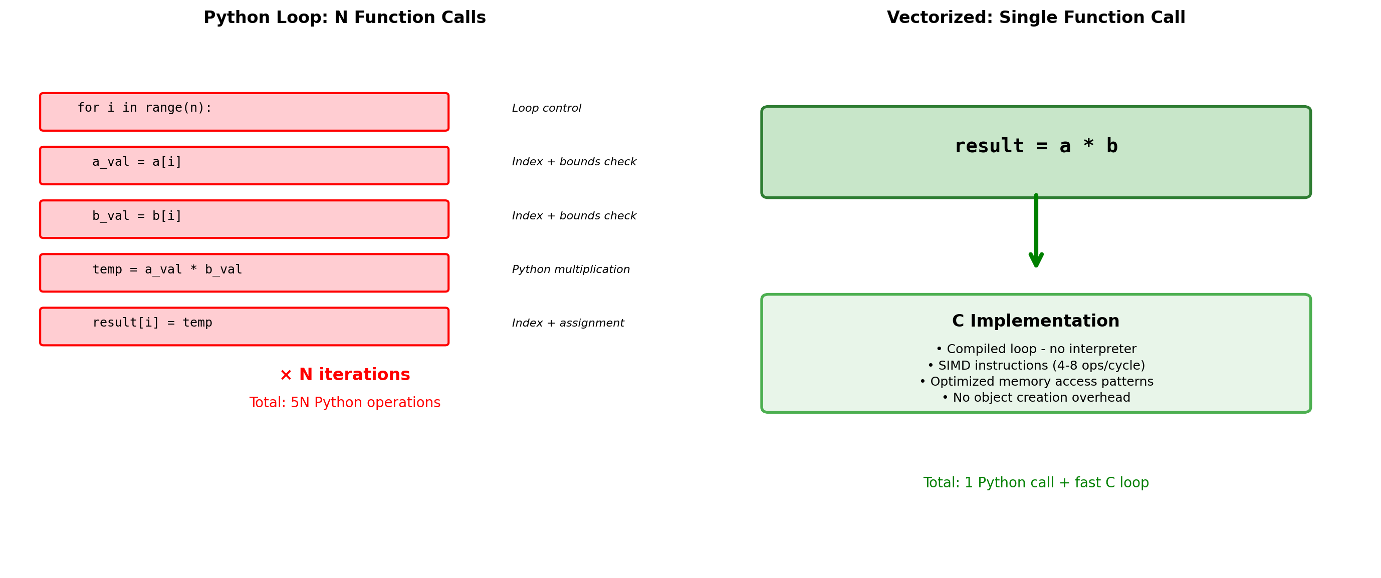
Vectorization: Moving Loops from Python to C
Vectorization replaces Python loops with single operations on entire arrays – significant performance increase.
import numpy as np
import timeit

# Demonstrate vectorization impact
def element_wise_python(a, b):
    """Element-wise operations in Python."""
    result = []
    for i in range(len(a)):
        result.append(a[i] * b[i] + 1.0)
    return result

def element_wise_vectorized(a, b):
    """Vectorized operations."""
    return a * b + 1.0

def mathematical_function_python(x):
    """Complex math in Python loop."""
    result = []
    for val in x:
        result.append(val**2 + np.sin(val) + np.exp(-val))
    return result

def mathematical_function_vectorized(x):
    """Complex math vectorized."""
    return x**2 + np.sin(x) + np.exp(-x)

# Performance comparison
sizes = [100, 1000, 10000, 100000]

print("Vectorization performance scaling:")
print("Size    | Python  | NumPy   | Speedup")
print("-" * 40)

for size in sizes:
    # Create test data
    a_list = [float(i) for i in range(size)]
    b_list = [float(i+1) for i in range(size)]
    a_array = np.array(a_list)
    b_array = np.array(b_list)

    # Reduce iterations for larger arrays
    iterations = max(1, 1000 // size)

    # Time Python version
    t_python = timeit.timeit(
        lambda: element_wise_python(a_list, b_list),
        number=iterations
    )

    # Time NumPy version
    t_numpy = timeit.timeit(
        lambda: element_wise_vectorized(a_array, b_array),
        number=iterations
    )

    speedup = t_python / t_numpy if t_numpy > 0 else float('inf')
    print(f"{size:5d}   | {t_python:.4f}  | {t_numpy:.4f}  | {speedup:5.0f}x")

# Complex mathematical operations
print(f"\nComplex mathematical functions (size 10,000):")
x_list = [i * 0.01 for i in range(10000)]
x_array = np.array(x_list)

t_math_python = timeit.timeit(
    lambda: mathematical_function_python(x_list),
    number=10
)

t_math_numpy = timeit.timeit(
    lambda: mathematical_function_vectorized(x_array),
    number=10
)

print(f"  Python loop: {t_math_python:.3f}s")
print(f"  Vectorized:  {t_math_numpy:.3f}s")
print(f"  Speedup: {t_math_python/t_math_numpy:.0f}x")

# Memory allocation overhead
def analyze_memory_pattern():
    """Show memory allocation in vectorized operations."""
    x = np.arange(1000000)

    # Multiple operations - intermediate arrays
    result1 = x * 2         # Creates intermediate array
    result2 = result1 + 1   # Creates another intermediate
    result3 = result2 ** 2  # Creates final result

    # Combined operation - fewer intermediates
    result_combined = (x * 2 + 1) ** 2

    return len([result1, result2, result3, result_combined])

print(f"\nMemory efficiency:")
print(f"  Intermediate arrays created in vectorized operations")
print(f"  Combine operations when possible: (x * 2 + 1) ** 2")
print(f"  vs separate: temp1 = x * 2; temp2 = temp1 + 1; result = temp2 ** 2")

# Function overhead demonstration
def tiny_function(x):
    return x + 1

x = np.arange(100000)

# Apply function element-wise (slow)
t_apply = timeit.timeit(
    lambda: np.array([tiny_function(val) for val in x]),
    number=10
)

# Vectorized equivalent (fast)
t_vector = timeit.timeit(
    lambda: x + 1,
    number=10
)

print(f"\nFunction call overhead (100,000 elements):")
print(f"  Element-wise function: {t_apply:.3f}s")
print(f"  Vectorized operation: {t_vector:.3f}s")
print(f"  Overhead cost: {t_apply/t_vector:.0f}x slower")
Vectorization performance scaling:
Size | Python | NumPy | Speedup
----------------------------------------
100 | 0.0000 | 0.0000 | 2x
1000 | 0.0000 | 0.0000 | 7x
10000 | 0.0003 | 0.0000 | 6x
100000 | 0.0027 | 0.0020 | 1x
Complex mathematical functions (size 10,000):
Python loop: 0.017s
Vectorized: 0.001s
Speedup: 29x
Memory efficiency:
Intermediate arrays created in vectorized operations
Combine operations when possible: (x * 2 + 1) ** 2
vs separate: temp1 = x * 2; temp2 = temp1 + 1; result = temp2 ** 2
Function call overhead (100,000 elements):
Element-wise function: 0.069s
Vectorized operation: 0.000s
Overhead cost: 476x slowerVectorization principles:
- Eliminate explicit loops - Let NumPy handle iteration in C
- Use array operations -
+,*,**work element-wise - Use NumPy functions -
np.sin(),np.exp()are vectorized - Minimize intermediate arrays - Combine operations when possible
- Avoid Python functions in loops - Function call overhead dominates
Advanced Indexing and Fancy Indexing
NumPy indexing extends beyond basic slicing to support boolean masks and integer arrays.
import numpy as np
import timeit

# Advanced indexing demonstration
data = np.arange(20).reshape(4, 5)
print("Original array:")
print(data)

# Boolean indexing
print("\nBoolean indexing (data > 10):")
mask = data > 10
print(f"Mask shape: {mask.shape}")
print(f"Result: {data[mask]}")  # Returns 1D array
print(f"Result shape: {data[mask].shape}")

# Fancy indexing with lists
print("\nFancy indexing with row selection:")
row_indices = [0, 2, 3]
selected_rows = data[row_indices]
print(f"Selected rows {row_indices}:")
print(selected_rows)

# 2D fancy indexing
print("\nFancy indexing for specific elements:")
rows = [0, 1, 2]
cols = [1, 3, 4]
elements = data[rows, cols]  # Selects (0,1), (1,3), (2,4)
print(f"Elements at (0,1), (1,3), (2,4): {elements}")

# Mixed indexing
print("\nMixed indexing (slice + fancy):")
mixed = data[:, [1, 3]]  # All rows, columns 1 and 3
print(mixed)

# Where function for conditional selection
print("\nUsing np.where for conditional operations:")
result = np.where(data > 10, data, 0)  # Replace values ≤10 with 0
print("Values > 10 kept, others become 0:")
print(result)

# Performance analysis
def compare_indexing_performance():
    """Compare different indexing approaches."""
    size = 100000
    arr = np.random.randint(0, 100, size)

    # Boolean indexing
    t_boolean = timeit.timeit(
        lambda: arr[arr > 50],
        number=100
    )

    # Fancy indexing
    indices = np.where(arr > 50)[0]
    t_fancy = timeit.timeit(
        lambda: arr[indices],
        number=100
    )

    # Basic slicing (for comparison)
    t_slice = timeit.timeit(
        lambda: arr[10000:20000],
        number=100
    )

    return t_boolean, t_fancy, t_slice

t_bool, t_fancy, t_slice = compare_indexing_performance()

print(f"\nIndexing performance (100,000 elements, 100 iterations):")
print(f"  Basic slicing: {t_slice:.3f}s (creates view)")
print(f"  Boolean indexing: {t_bool:.3f}s ({t_bool/t_slice:.0f}x slower)")
print(f"  Fancy indexing: {t_fancy:.3f}s ({t_fancy/t_slice:.0f}x slower)")

# Memory implications
large_array = np.random.rand(10000, 1000)
bool_mask = large_array > 0.5

print(f"\nMemory implications:")
print(f"  Original array: {large_array.nbytes / 1024**2:.1f} MB")
print(f"  Boolean mask: {bool_mask.nbytes / 1024**2:.1f} MB")
print(f"  Boolean result: {large_array[bool_mask].nbytes / 1024**2:.1f} MB")

# Advanced boolean operations
print(f"\nComplex boolean operations:")
arr = np.random.randint(0, 20, (5, 5))
print("Array:")
print(arr)

# Multiple conditions
complex_mask = (arr > 5) & (arr < 15)  # Element-wise AND
print(f"\nElements between 5 and 15: {arr[complex_mask]}")

# Any/all operations
print(f"Any element > 15: {np.any(arr > 15)}")
print(f"All elements > 0: {np.all(arr > 0)}")

# Axis-specific operations
print(f"Rows with any element > 15: {np.any(arr > 15, axis=1)}")
print(f"Columns with all elements > 5: {np.all(arr > 5, axis=0)}")
Original array:
[[ 0 1 2 3 4]
[ 5 6 7 8 9]
[10 11 12 13 14]
[15 16 17 18 19]]
Boolean indexing (data > 10):
Mask shape: (4, 5)
Result: [11 12 13 14 15 16 17 18 19]
Result shape: (9,)
Fancy indexing with row selection:
Selected rows [0, 2, 3]:
[[ 0 1 2 3 4]
[10 11 12 13 14]
[15 16 17 18 19]]
Fancy indexing for specific elements:
Elements at (0,1), (1,3), (2,4): [ 1 8 14]
Mixed indexing (slice + fancy):
[[ 1 3]
[ 6 8]
[11 13]
[16 18]]
Using np.where for conditional operations:
Values > 10 kept, others become 0:
[[ 0 0 0 0 0]
[ 0 0 0 0 0]
[ 0 11 12 13 14]
[15 16 17 18 19]]
Indexing performance (100,000 elements, 100 iterations):
Basic slicing: 0.000s (creates view)
Boolean indexing: 0.027s (4549x slower)
Fancy indexing: 0.002s (340x slower)
Memory implications:
Original array: 76.3 MB
Boolean mask: 9.5 MB
Boolean result: 38.1 MB
Complex boolean operations:
Array:
[[19 2 14 8 15]
[ 7 2 8 5 5]
[ 7 15 12 0 5]
[ 1 10 16 16 3]
[16 7 0 2 12]]
Elements between 5 and 15: [14 8 7 8 7 12 10 7 12]
Any element > 15: True
All elements > 0: False
Rows with any element > 15: [ True False False True True]
Columns with all elements > 5: [False False False False False]Indexing creates views vs copies:
- Basic slicing: Creates views (shares memory)
- Boolean indexing: Always creates copies
- Fancy indexing: Always creates copies
- Views are faster but copies are safer
Pseudorandom Number Generation
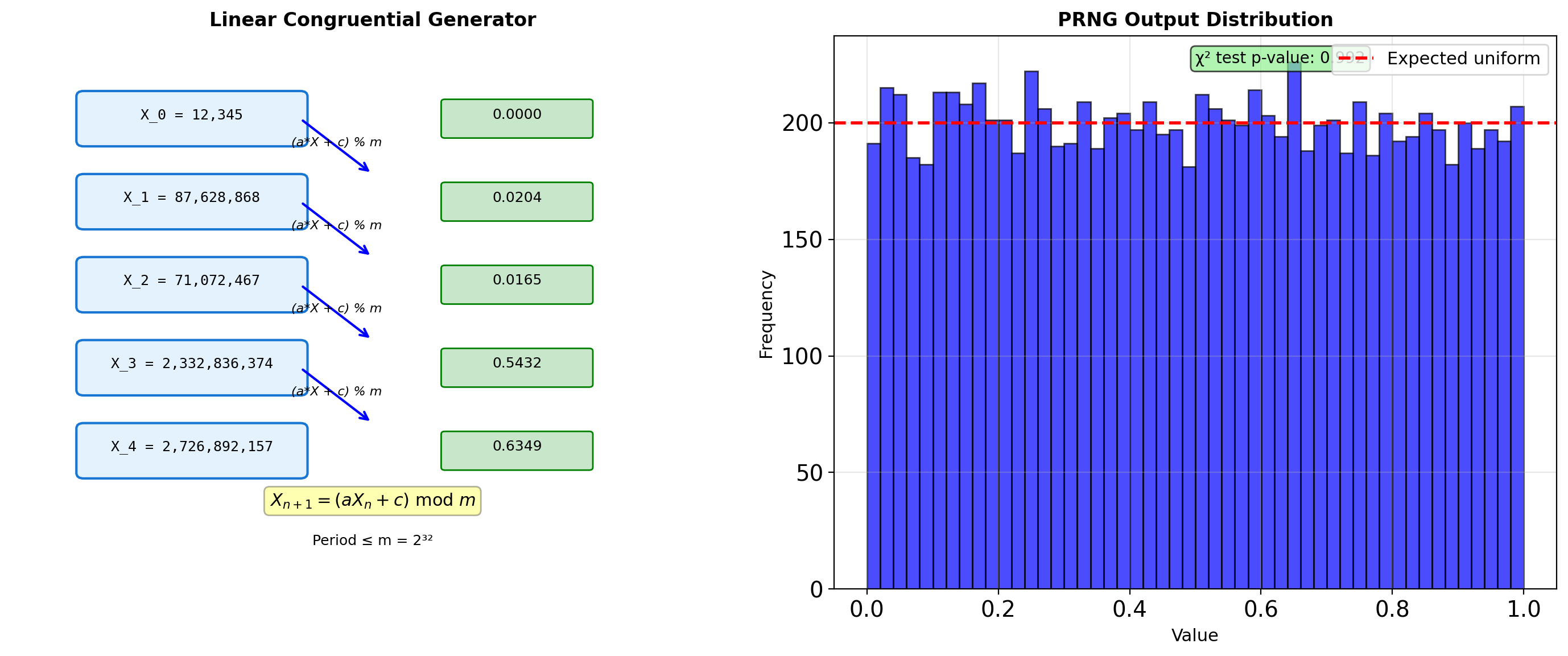
LCG (Linear Congruential Generator):
\[X_{n+1} = (aX_n + c) \mod m\]
- Simple, fast, but limited period (≤ m)
- Used historically; now superseded
Modern generator properties:
- Period: MT19937 has period 2^19937-1
- Quality: Pass TestU01 BigCrush (160 statistical tests)
- Speed: PCG64 is faster than MT19937
- State size: PCG64 uses 128 bits vs MT’s 19937 bits
PRNG output is deterministic given the seed — this enables reproducibility.
# Modern generators comparison
import numpy as np
import time

# Different PRNG algorithms
generators = {
    'PCG64': np.random.PCG64,
    'MT19937': np.random.MT19937,  # Mersenne Twister
    'Philox': np.random.Philox,
    'SFC64': np.random.SFC64,
}

print("Generator properties:")
for name, gen_class in generators.items():
    gen = np.random.Generator(gen_class(seed=42))

    # Generate samples for timing
    start = time.perf_counter()
    samples = gen.random(1000000)
    elapsed = time.perf_counter() - start

    print(f"\n{name}:")
    print(f"  Time for 1M: {elapsed:.3f}s")
    print(f"  Mean: {samples.mean():.6f}")
    print(f"  Std:  {samples.std():.6f}")

# State size comparison
mt = np.random.MT19937(seed=42)
pcg = np.random.PCG64(seed=42)

print(f"\nState size:")
print(f"  MT19937: {len(mt.state['state']['key'])} × 32 bits")
print(f"  PCG64: 2 × 64 bits")
Generator properties:
PCG64:
Time for 1M: 0.004s
Mean: 0.500026
Std: 0.288635
MT19937:
Time for 1M: 0.002s
Mean: 0.499778
Std: 0.288707
Philox:
Time for 1M: 0.003s
Mean: 0.499806
Std: 0.288525
SFC64:
Time for 1M: 0.003s
Mean: 0.499989
Std: 0.288734
State size:
MT19937: 624 × 32 bits
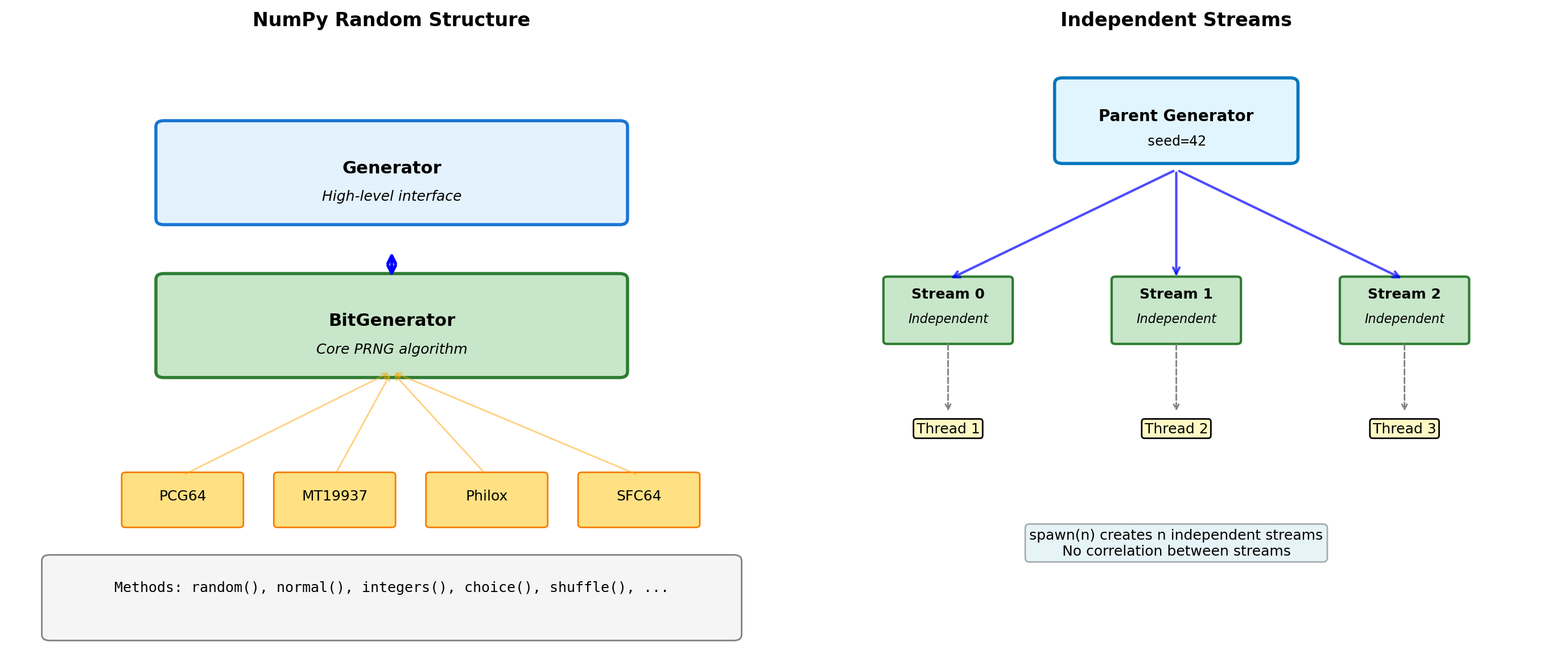
PCG64: 2 × 64 bitsNumPy Random Architecture

import numpy as np
# Modern NumPy random (v1.17+)
rng = np.random.default_rng(seed=42)
# Basic generation
print("Uniform [0, 1):", rng.random(5))
print("Integers [0, 10):", rng.integers(0, 10, size=5))
print("Normal(0, 1):", rng.normal(0, 1, size=5))
# Generator state management
initial_state = rng.bit_generator.state
# Generate some numbers
vals1 = rng.random(3)
print(f"\nFirst draw: {vals1}")
# Restore state
rng.bit_generator.state = initial_state
vals2 = rng.random(3)
print(f"After restore: {vals2}")
print(f"Same values: {np.array_equal(vals1, vals2)}")
# Spawn independent streams
parent_rng = np.random.default_rng(seed=42)
child_rngs = parent_rng.spawn(3)
print("\nIndependent streams:")
for i, child in enumerate(child_rngs):
print(f" Stream {i}: {child.random(3)}")Uniform [0, 1): [0.77395605 0.43887844 0.85859792 0.69736803 0.09417735]
Integers [0, 10): [5 9 7 7 7]
Normal(0, 1): [-0.01680116 -0.85304393 0.87939797 0.77779194 0.0660307 ]
First draw: [0.82276161 0.4434142 0.22723872]
After restore: [0.82276161 0.4434142 0.22723872]
Same values: True
Independent streams:
Stream 0: [0.91674416 0.91098667 0.8765925 ]
Stream 1: [0.46749078 0.0464489 0.59551001]
Stream 2: [0.0712392 0.71015972 0.07180046]# Performance: vectorized vs loop
import time
rng = np.random.default_rng(seed=42)
n = 1000000
# Vectorized generation
start = time.perf_counter()
vec_samples = rng.normal(0, 1, size=n)
vec_time = time.perf_counter() - start
# Loop generation
start = time.perf_counter()
loop_samples = [rng.normal(0, 1) for _ in range(n)]
loop_time = time.perf_counter() - start
print(f"Generation of {n:,} normals:")
print(f" Vectorized: {vec_time:.3f}s")
print(f" Loop: {loop_time:.3f}s")
print(f" Speedup: {loop_time/vec_time:.1f}x")
# Memory layout matters
print(f"\nMemory layout:")
print(f" Vectorized: {vec_samples.flags['C_CONTIGUOUS']}")
print(f" Array strides: {vec_samples.strides}")
# Custom distribution via inverse transform
def exponential_inverse_transform(rng, rate, size):
"""Generate exponential via inverse CDF."""
u = rng.random(size)
return -np.log(1 - u) / rate
custom_exp = exponential_inverse_transform(rng, rate=2.0, size=1000)
numpy_exp = rng.exponential(scale=0.5, size=1000)
print(f"\nCustom vs NumPy exponential:")
print(f" Custom mean: {custom_exp.mean():.3f}")
print(f" NumPy mean: {numpy_exp.mean():.3f}")
print(f" Theoretical: {0.5:.3f}")Generation of 1,000,000 normals:
Vectorized: 0.004s
Loop: 0.306s
Speedup: 73.2x
Memory layout:
Vectorized: True
Array strides: (8,)
Custom vs NumPy exponential:
Custom mean: 0.507
NumPy mean: 0.497
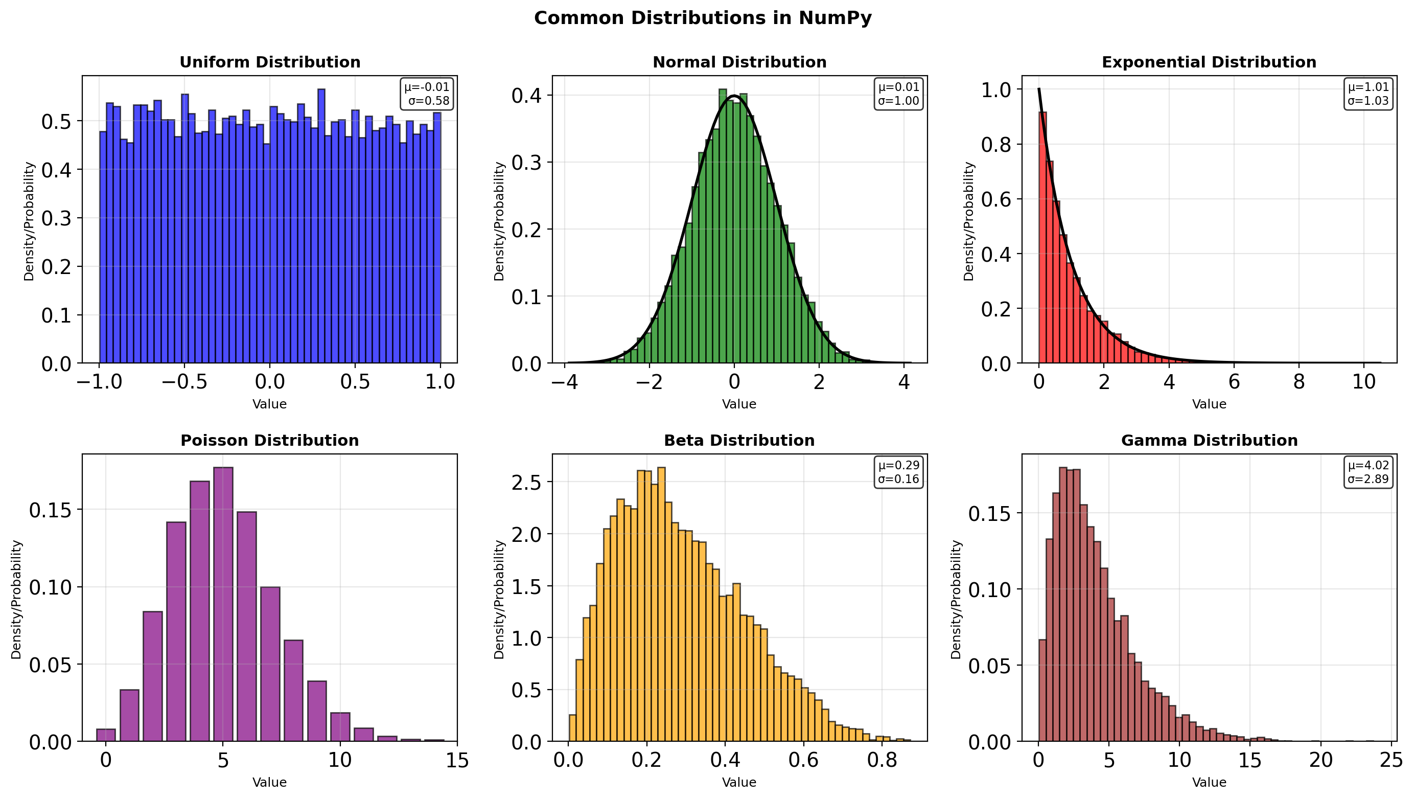
Theoretical: 0.500Distribution Sampling

import numpy as np
from scipy import stats
rng = np.random.default_rng(seed=42)
# Sampling from various distributions
n = 1000
# Continuous distributions
uniform = rng.uniform(low=0, high=10, size=n)
normal = rng.normal(loc=100, scale=15, size=n)
exponential = rng.exponential(scale=2.0, size=n)
gamma = rng.gamma(shape=2, scale=2, size=n)
# Discrete distributions
poisson = rng.poisson(lam=3, size=n)
binomial = rng.binomial(n=10, p=0.3, size=n)
print("Sample statistics:")
print(f"Uniform[0,10]: μ={uniform.mean():.2f}, σ={uniform.std():.2f}")
print(f"Normal(100,15): μ={normal.mean():.2f}, σ={normal.std():.2f}")
print(f"Exponential(2): μ={exponential.mean():.2f}, σ={exponential.std():.2f}")
print(f"Poisson(3): μ={poisson.mean():.2f}, σ={poisson.std():.2f}")
# Multivariate distributions
mean = [0, 0]
cov = [[1, 0.5], [0.5, 1]]
multivariate = rng.multivariate_normal(mean, cov, size=1000)
print(f"\nMultivariate normal:")
print(f" Shape: {multivariate.shape}")
print(f" Correlation: {np.corrcoef(multivariate.T)[0,1]:.3f}")Sample statistics:
Uniform[0,10]: μ=4.97, σ=2.91
Normal(100,15): μ=98.83, σ=15.21
Exponential(2): μ=1.97, σ=1.96
Poisson(3): μ=2.97, σ=1.75
Multivariate normal:
Shape: (1000, 2)
Correlation: 0.459# Transformation methods
rng = np.random.default_rng(seed=42)
# Box-Muller transform for normal
def box_muller(rng, size):
"""Generate normal(0,1) from uniform."""
u1 = rng.random(size)
u2 = rng.random(size)
z0 = np.sqrt(-2 * np.log(u1)) * np.cos(2 * np.pi * u2)
z1 = np.sqrt(-2 * np.log(u1)) * np.sin(2 * np.pi * u2)
return z0, z1
z0, z1 = box_muller(rng, 5000)
print(f"Box-Muller normal:")
print(f" Mean: {z0.mean():.3f}, {z1.mean():.3f}")
print(f" Std: {z0.std():.3f}, {z1.std():.3f}")
# Rejection sampling for arbitrary distribution
def rejection_sample(pdf, bounds, rng, n_samples):
"""Sample from arbitrary PDF via rejection."""
samples = []
low, high = bounds
# Find maximum of PDF for efficiency
x_test = np.linspace(low, high, 1000)
max_pdf = np.max([pdf(x) for x in x_test])
while len(samples) < n_samples:
x = rng.uniform(low, high)
y = rng.uniform(0, max_pdf)
if y <= pdf(x):
samples.append(x)
return np.array(samples)
# Sample from beta-like distribution
pdf = lambda x: 2 * x if 0 <= x <= 1 else 0
samples = rejection_sample(pdf, (0, 1), rng, 1000)
print(f"\nRejection sampling:")
print(f" Mean: {samples.mean():.3f} (theory: 0.667)")Box-Muller normal:
Mean: -0.005, 0.000
Std: 1.002, 1.005
Rejection sampling:
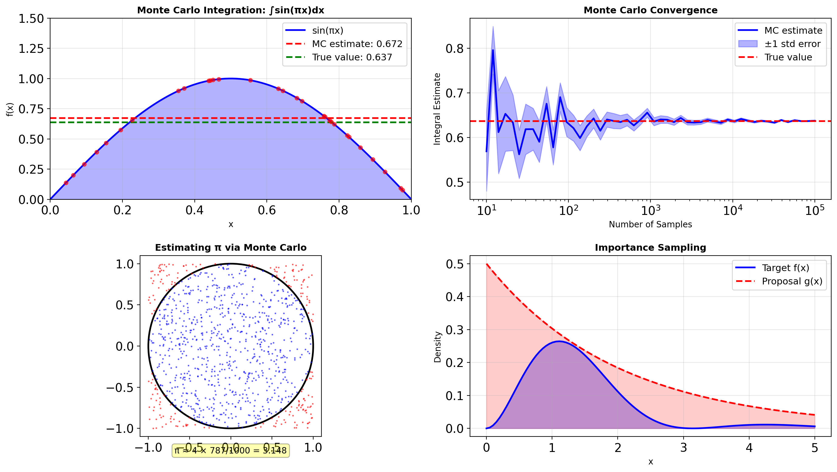
Mean: 0.666 (theory: 0.667)Monte Carlo Integration
import numpy as np
def monte_carlo_integrate(func, bounds, n_samples, rng=None):
"""Basic Monte Carlo integration."""
if rng is None:
rng = np.random.default_rng()
a, b = bounds
# Sample uniformly in domain
x = rng.uniform(a, b, n_samples)
# Evaluate function
y = func(x)
# MC estimate: (b-a) * mean(f)
integral = (b - a) * np.mean(y)
std_error = (b - a) * np.std(y) / np.sqrt(n_samples)
return integral, std_error
# Example: ∫₀¹ sin(πx) dx = 2/π
rng = np.random.default_rng(seed=42)
for n in [100, 1000, 10000, 100000]:
integral, error = monte_carlo_integrate(
lambda x: np.sin(np.pi * x),
bounds=(0, 1),
n_samples=n,
rng=rng
)
true_value = 2/np.pi
print(f"n={n:6d}: {integral:.5f} ± {error:.5f} (true: {true_value:.5f})")
# Multidimensional integration
def monte_carlo_nd(func, bounds, n_samples, rng=None):
"""N-dimensional Monte Carlo integration."""
if rng is None:
rng = np.random.default_rng()
ndim = len(bounds)
volume = np.prod([b - a for a, b in bounds])
# Sample in hypercube
samples = np.zeros((n_samples, ndim))
for i, (a, b) in enumerate(bounds):
samples[:, i] = rng.uniform(a, b, n_samples)
# Evaluate function
values = np.array([func(*s) for s in samples])
integral = volume * np.mean(values)
std_error = volume * np.std(values) / np.sqrt(n_samples)
return integral, std_error
# 2D example: ∫∫ exp(-(x²+y²)) dx dy over unit square
def gaussian_2d(x, y):
return np.exp(-(x**2 + y**2))
integral_2d, error_2d = monte_carlo_nd(
gaussian_2d,
bounds=[(0, 1), (0, 1)],
n_samples=10000,
rng=rng
)
print(f"\n2D integral: {integral_2d:.5f} ± {error_2d:.5f}")n= 100: 0.67226 ± 0.02825 (true: 0.63662)
n= 1000: 0.63032 ± 0.00972 (true: 0.63662)
n= 10000: 0.63801 ± 0.00308 (true: 0.63662)
n=100000: 0.63706 ± 0.00097 (true: 0.63662)
2D integral: 0.55976 ± 0.00217# Variance reduction: stratified sampling
def stratified_monte_carlo(func, bounds, n_strata, samples_per_stratum, rng=None):
"""Stratified Monte Carlo for variance reduction."""
if rng is None:
rng = np.random.default_rng()
a, b = bounds
stratum_width = (b - a) / n_strata
estimates = []
for i in range(n_strata):
# Sample within stratum
stratum_a = a + i * stratum_width
stratum_b = a + (i + 1) * stratum_width
x = rng.uniform(stratum_a, stratum_b, samples_per_stratum)
y = func(x)
# Stratum estimate
estimates.append(np.mean(y))
# Combine strata
integral = (b - a) * np.mean(estimates)
std_error = (b - a) * np.std(estimates) / np.sqrt(n_strata)
return integral, std_error
# Compare standard vs stratified
n_total = 10000
# Standard MC
standard_int, standard_err = monte_carlo_integrate(
lambda x: np.sin(np.pi * x),
bounds=(0, 1),
n_samples=n_total,
rng=rng
)
# Stratified MC
n_strata = 100
stratified_int, stratified_err = stratified_monte_carlo(
lambda x: np.sin(np.pi * x),
bounds=(0, 1),
n_strata=n_strata,
samples_per_stratum=n_total // n_strata,
rng=rng
)
print(f"Variance reduction comparison ({n_total} samples):")
print(f" Standard: {standard_int:.5f} ± {standard_err:.5f}")
print(f" Stratified: {stratified_int:.5f} ± {stratified_err:.5f}")
print(f" Error reduction: {standard_err/stratified_err:.2f}x")Variance reduction comparison (10000 samples):
Standard: 0.63776 ± 0.00306
Stratified: 0.63655 ± 0.03078
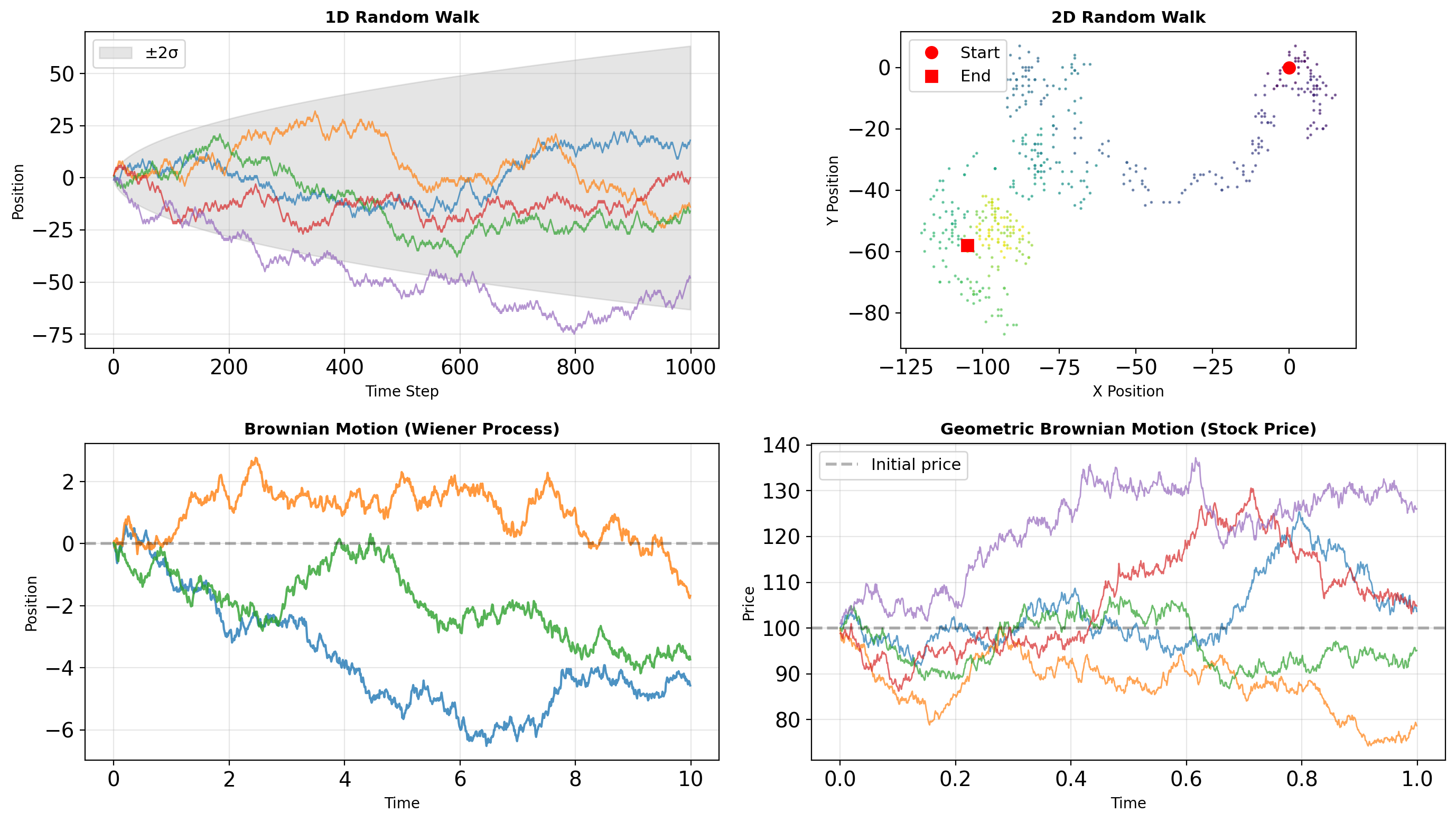
Error reduction: 0.10xRandom Walks and Stochastic Processes
import numpy as np
class RandomWalk:
"""1D and 2D random walk simulator."""
def __init__(self, seed=None):
self.rng = np.random.default_rng(seed)
def walk_1d(self, n_steps, p_up=0.5):
"""1D random walk with bias."""
steps = self.rng.choice(
[-1, 1],
size=n_steps,
p=[1-p_up, p_up]
)
return np.cumsum(steps)
def walk_2d(self, n_steps):
"""2D random walk on lattice."""
# Possible moves: up, down, left, right
moves = np.array([[0, 1], [0, -1], [-1, 0], [1, 0]])
choices = self.rng.integers(0, 4, size=n_steps)
steps = moves[choices]
path = np.cumsum(steps, axis=0)
return path[:, 0], path[:, 1]
def first_passage_time(self, barrier, max_steps=10000):
"""Time to first reach barrier."""
position = 0
for step in range(max_steps):
position += self.rng.choice([-1, 1])
if abs(position) >= barrier:
return step + 1
return None
# Analyze random walk properties
walker = RandomWalk(seed=42)
# First passage times
barriers = [10, 20, 50]
n_trials = 1000
for barrier in barriers:
times = []
for _ in range(n_trials):
t = walker.first_passage_time(barrier)
if t is not None:
times.append(t)
mean_time = np.mean(times)
theoretical = barrier ** 2 # E[T] = n² for symmetric walk
print(f"Barrier ±{barrier}:")
print(f" Mean time: {mean_time:.1f}")
print(f" Theory: {theoretical:.1f}")
print(f" Success rate: {len(times)/n_trials:.1%}")Barrier ±10:
Mean time: 99.2
Theory: 100.0
Success rate: 100.0%
Barrier ±20:
Mean time: 405.9
Theory: 400.0
Success rate: 100.0%
Barrier ±50:
Mean time: 2384.1
Theory: 2500.0
Success rate: 99.3%# Stochastic differential equations
def euler_maruyama(sde_drift, sde_diffusion, x0, t_span, dt, rng=None):
"""Solve SDE using Euler-Maruyama method."""
if rng is None:
rng = np.random.default_rng()
t = np.arange(t_span[0], t_span[1], dt)
n = len(t)
x = np.zeros(n)
x[0] = x0
# Generate all random increments at once
dW = rng.normal(0, np.sqrt(dt), n-1)
for i in range(n-1):
drift = sde_drift(x[i], t[i])
diffusion = sde_diffusion(x[i], t[i])
x[i+1] = x[i] + drift*dt + diffusion*dW[i]
return t, x
# Ornstein-Uhlenbeck process (mean-reverting)
def ou_drift(x, t, theta=1.0, mu=0.0):
return theta * (mu - x)
def ou_diffusion(x, t, sigma=0.3):
return sigma
rng = np.random.default_rng(seed=42)
# Simulate multiple paths
print("Ornstein-Uhlenbeck process:")
for x0 in [2.0, 0.0, -2.0]:
t, x = euler_maruyama(
ou_drift, ou_diffusion,
x0=x0, t_span=(0, 10), dt=0.01,
rng=rng
)
print(f" Start: {x0:+.1f}, End: {x[-1]:+.2f}, Mean: {x[len(x)//2:].mean():+.2f}")
# Geometric Brownian Motion
def gbm_drift(S, t, mu=0.05):
return mu * S
def gbm_diffusion(S, t, sigma=0.2):
return sigma * S
t, S = euler_maruyama(
gbm_drift, gbm_diffusion,
x0=100, t_span=(0, 1), dt=0.001,
rng=rng
)
print(f"\nGBM Stock simulation:")
print(f" Initial: ${S[0]:.2f}")
print(f" Final: ${S[-1]:.2f}")
print(f" Return: {(S[-1]/S[0] - 1)*100:.1f}%")Ornstein-Uhlenbeck process:
Start: +2.0, End: +0.05, Mean: -0.15
Start: +0.0, End: -0.57, Mean: -0.38
Start: -2.0, End: +0.19, Mean: +0.13
GBM Stock simulation:
Initial: $100.00
Final: $104.77
Return: 4.8%Reproducibility and Parallel Streams

import numpy as np
from concurrent.futures import ProcessPoolExecutor
import multiprocessing as mp
def monte_carlo_pi(n_samples, seed):
"""Estimate π using Monte Carlo."""
rng = np.random.default_rng(seed)
# Generate points in unit square
x = rng.random(n_samples)
y = rng.random(n_samples)
# Count points inside circle
inside = (x**2 + y**2) <= 1
pi_estimate = 4 * inside.sum() / n_samples
return pi_estimate
# Serial execution
rng_main = np.random.default_rng(seed=42)
n_trials = 4
n_samples = 1000000
print("Serial execution:")
serial_results = []
for i in range(n_trials):
# Use different seed for each trial
seed = rng_main.integers(0, 2**32)
result = monte_carlo_pi(n_samples, seed)
serial_results.append(result)
print(f" Trial {i}: π ≈ {result:.5f}")
print(f" Mean: {np.mean(serial_results):.5f}")
print(f" Std: {np.std(serial_results):.5f}")
# Parallel execution with spawned generators
def parallel_monte_carlo():
"""Parallel MC with independent streams."""
parent_rng = np.random.default_rng(seed=42)
# Spawn independent streams
n_workers = mp.cpu_count()
child_seeds = parent_rng.spawn(n_workers)
# Create tasks with independent seeds
tasks = []
for i in range(n_workers):
# Extract seed value from SeedSequence
seed_value = child_seeds[i].generate_state(1)[0]
tasks.append((n_samples, seed_value))
return tasks
# Note: ProcessPoolExecutor not shown due to execution environment
print(f"\nParallel setup for {mp.cpu_count()} cores created")Serial execution:
Trial 0: π ≈ 3.14089
Trial 1: π ≈ 3.14045
Trial 2: π ≈ 3.14242
Trial 3: π ≈ 3.14100
Mean: 3.14119
Std: 0.00074
Parallel setup for 10 cores createdReproducibility patterns:
# Use explicit generators (not global state)
rng = np.random.default_rng(seed=42)
# Pass rng to functions explicitly
def simulate(n, rng):
return rng.normal(0, 1, n)
# Save/restore state for checkpoints
state = rng.bit_generator.state
# ... do work ...
rng.bit_generator.state = state # restore
# Use spawn() for parallel work
children = rng.spawn(4) # 4 independent streamsAvoid:
np.random.seed()— global state, not thread-safe- Creating
default_rng()without seed inside loops
Same seed + same code = identical results.
Lambda Functions: Anonymous Functions in Python
# Lambda basics
square = lambda x: x**2
add = lambda x, y: x + y
magnitude = lambda v: sum(x**2 for x in v) ** 0.5
print(f"square(5) = {square(5)}")
print(f"add(3, 4) = {add(3, 4)}")
print(f"magnitude([3, 4]) = {magnitude([3, 4])}")
# Lambda limitations - no statements
try:
# This won't work - assignment is a statement
bad_lambda = lambda x: (y := x + 1, y * 2)
except SyntaxError as e:
print(f"\nSyntax error in lambda")
# Workaround using expression forms
result = (lambda x: (x + 1) * 2)(5)
print(f"Workaround result: {result}")
# Lambda with conditional expression
abs_val = lambda x: x if x >= 0 else -x
sign = lambda x: 1 if x > 0 else (-1 if x < 0 else 0)
print(f"\nabs_val(-5) = {abs_val(-5)}")
print(f"sign(-5) = {sign(-5)}")
print(f"sign(0) = {sign(0)}")
print(f"sign(5) = {sign(5)}")square(5) = 25
add(3, 4) = 7
magnitude([3, 4]) = 5.0
Workaround result: 12
abs_val(-5) = 5
sign(-5) = -1
sign(0) = 0
sign(5) = 1# Lambdas in data processing
import numpy as np
# Sorting with custom key
points = [(3, 4), (1, 2), (5, 1), (2, 3)]
# Sort by distance from origin
by_distance = sorted(points, key=lambda p: (p[0]**2 + p[1]**2)**0.5)
print(f"By distance: {by_distance}")
# Sort by second coordinate
by_y = sorted(points, key=lambda p: p[1])
print(f"By y-coord: {by_y}")
# Complex sorting - primary and secondary keys
data = [('Alice', 85), ('Bob', 92), ('Charlie', 85), ('David', 78)]
sorted_data = sorted(data, key=lambda x: (-x[1], x[0]))
print(f"\nBy score desc, then name:")
for name, score in sorted_data:
print(f" {name}: {score}")
# Lambda in numerical operations
vectors = np.array([[1, 2], [3, 4], [5, 6]])
# Apply transformation
transform = lambda v: v / np.linalg.norm(v)
normalized = np.apply_along_axis(transform, 1, vectors)
print(f"\nNormalized vectors:")
print(normalized)By distance: [(1, 2), (2, 3), (3, 4), (5, 1)]
By y-coord: [(5, 1), (1, 2), (2, 3), (3, 4)]
By score desc, then name:
Bob: 92
Alice: 85
Charlie: 85
David: 78
Normalized vectors:
[[0.4472136 0.89442719]
[0.6 0.8 ]
[0.6401844 0.76822128]]Lambda Performance and Pitfalls

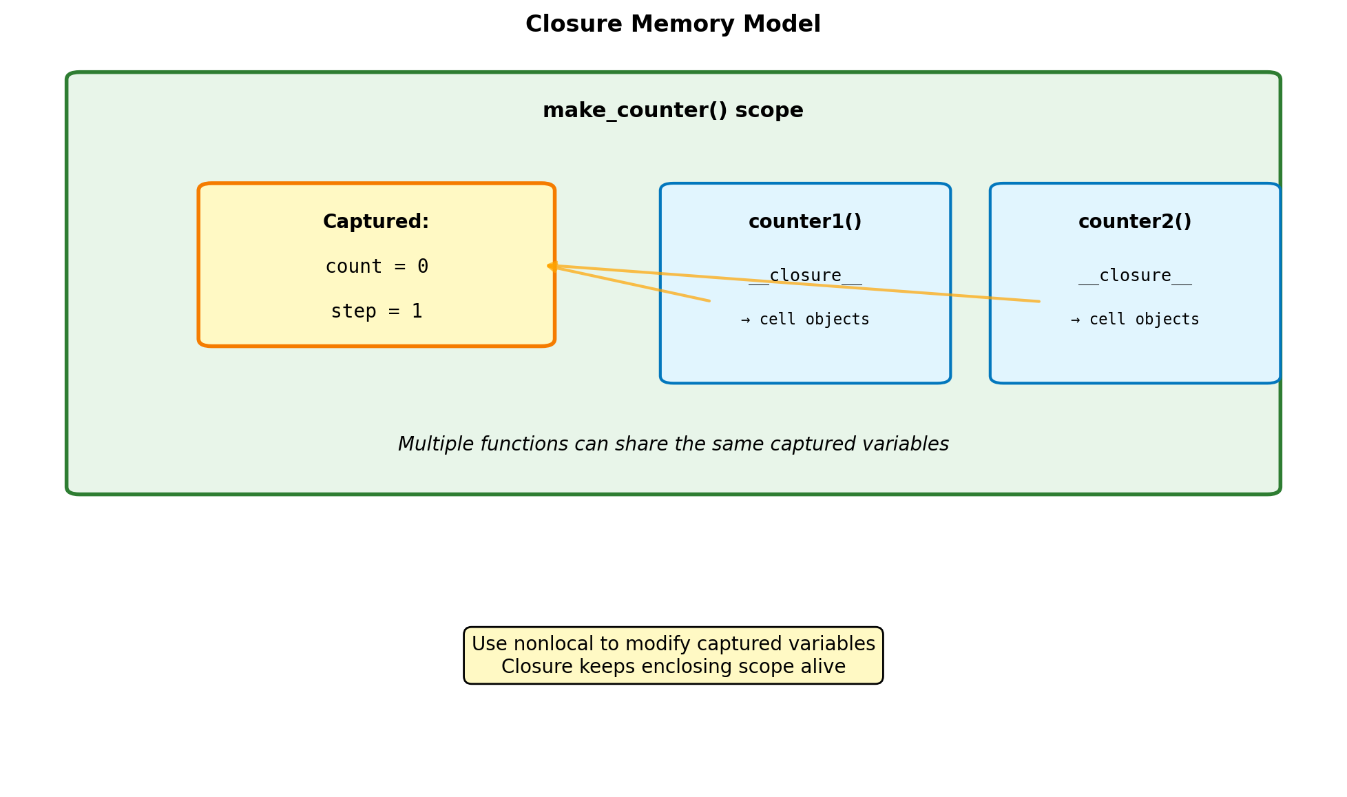
# Closure pitfall demonstration
print("Closure problem:")
funcs_bad = []
for i in range(3):
funcs_bad.append(lambda x: x + i)
# All functions use final value of i
for j, f in enumerate(funcs_bad):
print(f" func[{j}](10) = {f(10)}") # All return 12!
print("\nFixed with default argument:")
funcs_good = []
for i in range(3):
funcs_good.append(lambda x, i=i: x + i)
for j, f in enumerate(funcs_good):
print(f" func[{j}](10) = {f(10)}") # Correct: 10, 11, 12
# Alternative: use functools.partial
from functools import partial
def add(x, y):
return x + y
print("\nUsing partial:")
funcs_partial = [partial(add, y=i) for i in range(3)]
for j, f in enumerate(funcs_partial):
print(f" func[{j}](10) = {f(10)}")Closure problem:
func[0](10) = 12
func[1](10) = 12
func[2](10) = 12
Fixed with default argument:
func[0](10) = 10
func[1](10) = 11
func[2](10) = 12
Using partial:
func[0](10) = 10
func[1](10) = 11
func[2](10) = 12Closure capture rule:
Closures capture references to variables, not values. The variable is looked up when the function is called, not when it’s defined.
Fixes:
- Default argument:
lambda x, i=i: x + i functools.partial: binds value at creation time- Nested function with local binding
When lambdas are appropriate:
- Short, single-expression functions
- Throwaway functions for
sort,map,filter - Simple callbacks
Prefer named functions when:
- Logic is complex or reusable
- You need docstrings or type hints
- Debugging is important (lambdas have no name)
Map, Filter, Reduce: Functional Transformations
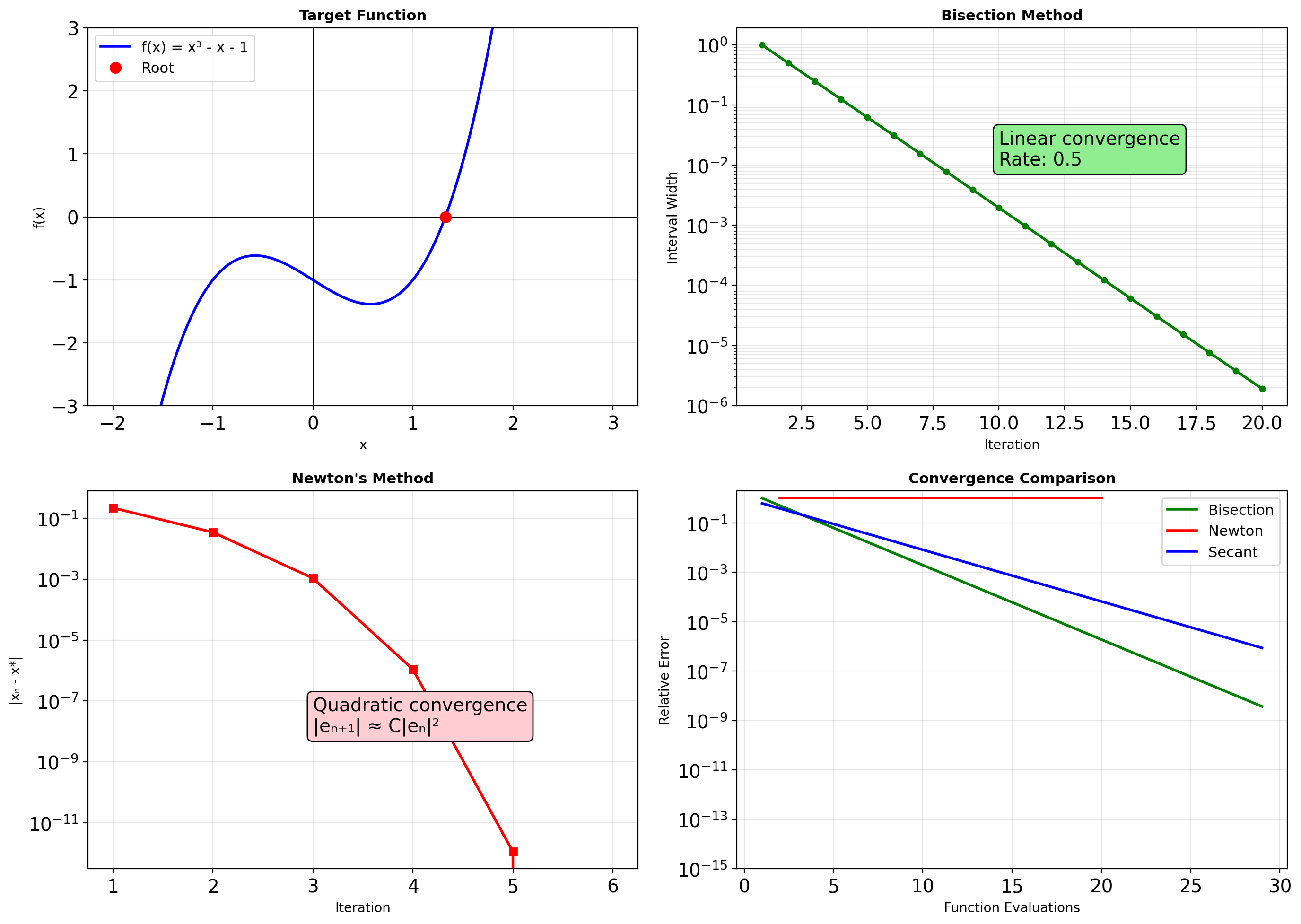
from functools import reduce
import operator
data = [1, 2, 3, 4, 5]
# Map: transform each element
squared = list(map(lambda x: x**2, data))
print(f"Original: {data}")
print(f"Squared: {squared}")
# Filter: select elements
evens = list(filter(lambda x: x % 2 == 0, data))
odds = list(filter(lambda x: x % 2 == 1, data))
print(f"\nEvens: {evens}")
print(f"Odds: {odds}")
# Reduce: accumulate to single value
sum_all = reduce(operator.add, data)
product = reduce(operator.mul, data)
max_val = reduce(lambda a, b: a if a > b else b, data)
print(f"\nSum: {sum_all}")
print(f"Product: {product}")
print(f"Max: {max_val}")
# Combining operations
result = reduce(
operator.add,
filter(
lambda x: x > 10,
map(lambda x: x**2, data)
)
)
print(f"\nSum of squares > 10: {result}")
# Functional pipeline
def pipeline(data, *functions):
"""Apply functions in sequence."""
for func in functions:
data = func(data)
return data
result = pipeline(
range(10),
lambda x: map(lambda n: n**2, x),
lambda x: filter(lambda n: n % 2 == 0, x),
list
)
print(f"\nPipeline result: {result}")Original: [1, 2, 3, 4, 5]
Squared: [1, 4, 9, 16, 25]
Evens: [2, 4]
Odds: [1, 3, 5]
Sum: 15
Product: 120
Max: 5
Sum of squares > 10: 41
Pipeline result: [0, 4, 16, 36, 64]# Performance comparison
import timeit
import numpy as np
data = list(range(1000))
# Map alternatives
t_map = timeit.timeit(
lambda: list(map(lambda x: x**2, data)),
number=1000
)
t_comp = timeit.timeit(
lambda: [x**2 for x in data],
number=1000
)
t_numpy = timeit.timeit(
lambda: np.array(data)**2,
number=1000
)
print(f"Squaring 1000 numbers:")
print(f" map(): {t_map:.3f}s")
print(f" List comp: {t_comp:.3f}s ({t_map/t_comp:.2f}x)")
print(f" NumPy: {t_numpy:.3f}s ({t_map/t_numpy:.1f}x)")
# Memory efficiency
print(f"\nMemory behavior:")
# Map returns iterator (lazy)
mapped = map(lambda x: x**2, range(1000000))
print(f" map object: {sys.getsizeof(mapped)} bytes")
# List comprehension creates full list
comp = [x**2 for x in range(100000)] # Smaller for memory
print(f" List comp (100k): {sys.getsizeof(comp):,} bytes")
# Generator expression (lazy like map)
gen = (x**2 for x in range(1000000))
print(f" Generator expr: {sys.getsizeof(gen)} bytes")
# Practical reduce example
from itertools import accumulate
# Running statistics
values = [3, 1, 4, 1, 5, 9, 2, 6]
running_sum = list(accumulate(values))
running_max = list(accumulate(values, max))
print(f"\nValues: {values}")
print(f"Running sum: {running_sum}")
print(f"Running max: {running_max}")Squaring 1000 numbers:
map(): 0.028s
List comp: 0.017s (1.69x)
NumPy: 0.023s (1.2x)
Memory behavior:
map object: 48 bytes
List comp (100k): 800,984 bytes
Generator expr: 200 bytes
Values: [3, 1, 4, 1, 5, 9, 2, 6]
Running sum: [3, 4, 8, 9, 14, 23, 25, 31]
Running max: [3, 3, 4, 4, 5, 9, 9, 9]Map, Filter, Reduce in Numerical Computing
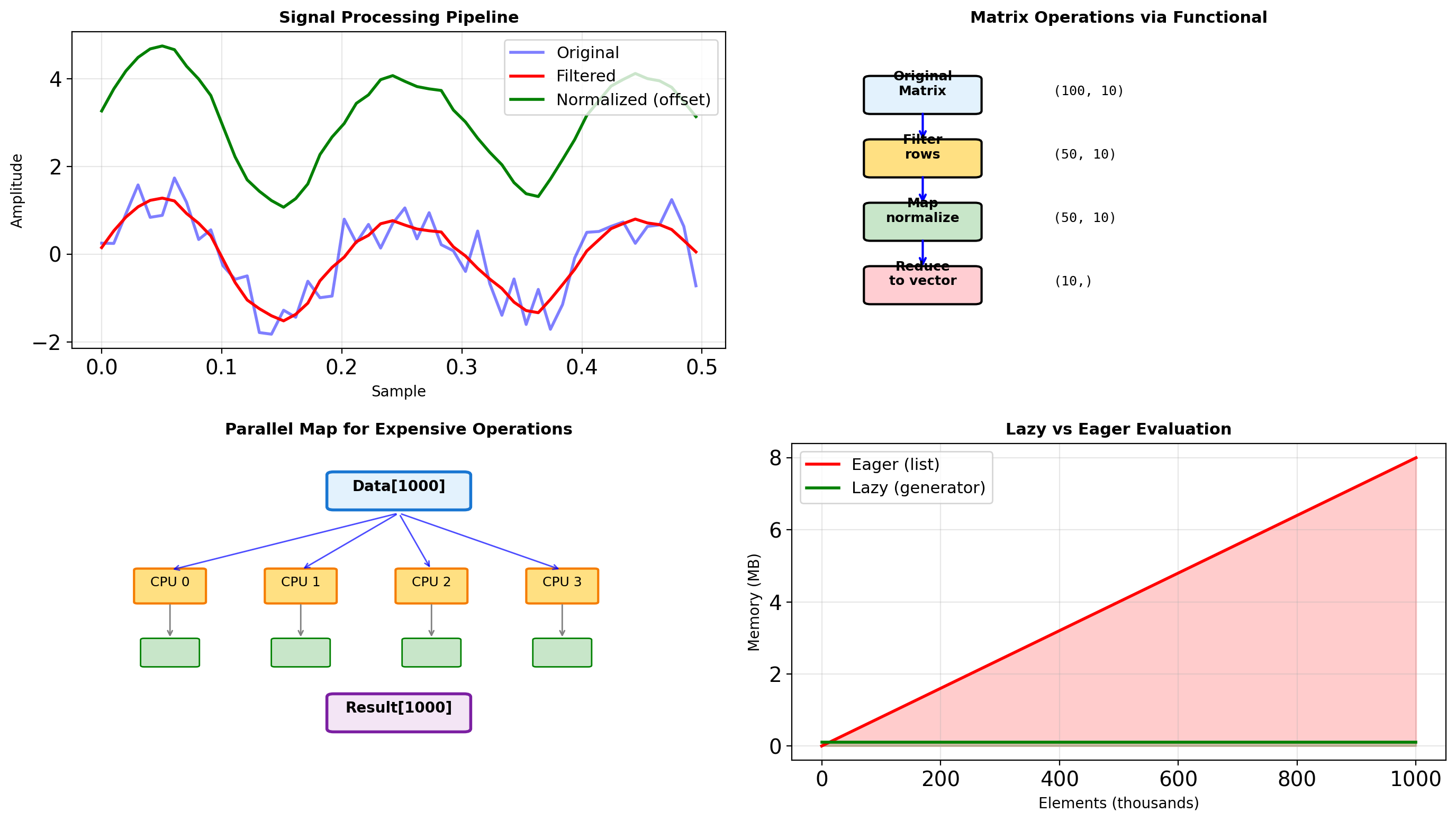
import numpy as np
from functools import reduce
# Signal processing pipeline
def process_signals(signals):
"""Functional signal processing pipeline."""
# Filter: remove invalid signals
valid = filter(lambda s: not np.any(np.isnan(s)), signals)
# Map: normalize each signal
normalized = map(lambda s: (s - s.mean()) / s.std(), valid)
# Map: compute features
features = map(lambda s: {
'energy': np.sum(s**2),
'peak': np.max(np.abs(s)),
'zero_crossings': np.sum(np.diff(np.sign(s)) != 0)
}, normalized)
return list(features)
# Generate test signals
np.random.seed(42)
signals = [
np.sin(np.linspace(0, 2*np.pi, 100)) + 0.1*np.random.randn(100),
np.random.randn(100),
np.array([np.nan] * 100), # Invalid
np.cos(np.linspace(0, 4*np.pi, 100)),
]
results = process_signals(signals)
print("Signal features:")
for i, feat in enumerate(results):
print(f" Signal {i}: energy={feat['energy']:.1f}, "
f"peak={feat['peak']:.2f}, crossings={feat['zero_crossings']}")
# Matrix operations with functional approach
def matrix_pipeline(matrix):
"""Process matrix rows functionally."""
# Filter rows by condition
filtered_rows = filter(
lambda row: np.sum(row) > 0,
matrix
)
# Normalize each row
normalized = map(
lambda row: row / np.linalg.norm(row),
filtered_rows
)
# Reduce to summary statistics
row_list = list(normalized)
if row_list:
mean_row = reduce(
lambda a, b: a + b,
row_list
) / len(row_list)
return mean_row
return None
# Test matrix
matrix = np.random.randn(10, 5)
matrix[2] = -np.abs(matrix[2]) # Make one row negative sum
result = matrix_pipeline(matrix)
print(f"\nMean normalized row: {result}")Signal features:
Signal 0: energy=100.0, peak=1.80, crossings=3
Signal 1: energy=100.0, peak=2.84, crossings=54
Signal 2: energy=100.0, peak=1.42, crossings=4
Mean normalized row: [ 0.01159341 0.05561288 -0.05330941 0.1654067 0.35741119]# Parallel map for expensive operations
from multiprocessing import Pool
import time
def expensive_computation(x):
"""Simulate expensive computation."""
# In real code, this might be optimization, simulation, etc.
result = 0
for i in range(100000):
result += x * np.sin(i) * np.cos(i)
return result / 100000
# Sequential map
data = list(range(10))
start = time.perf_counter()
sequential_results = list(map(expensive_computation, data))
seq_time = time.perf_counter() - start
print(f"Sequential map: {seq_time:.3f}s")
# Parallel map (simplified for demonstration)
# Note: In Jupyter/interactive environments, use:
# from multiprocessing.dummy import Pool # Thread pool
# Or restructure for subprocess pool
def parallel_map(func, data, n_workers=4):
"""Simple parallel map implementation."""
# Simulate parallel execution
# In production, use multiprocessing.Pool
results = []
chunk_size = len(data) // n_workers
for i in range(0, len(data), chunk_size):
chunk = data[i:i+chunk_size]
results.extend(map(func, chunk))
return results
# Lazy evaluation for large datasets
def lazy_pipeline(data_generator):
"""Process infinite/large data streams."""
# Chain of transformations (all lazy)
transformed = map(lambda x: x**2, data_generator)
filtered = filter(lambda x: x % 2 == 0, transformed)
processed = map(lambda x: x // 2, filtered)
# Only compute what's needed
return processed
# Infinite generator
def fibonacci():
a, b = 0, 1
while True:
yield a
a, b = b, a + b
# Process only first 10 values
pipeline = lazy_pipeline(fibonacci())
first_10 = [next(pipeline) for _ in range(10)]
print(f"\nFirst 10 processed Fibonacci: {first_10}")
# Memory comparison
import sys
eager_list = [x**2 for x in range(100000)]
lazy_gen = (x**2 for x in range(100000))
print(f"\nMemory usage:")
print(f" Eager list: {sys.getsizeof(eager_list):,} bytes")
print(f" Lazy generator: {sys.getsizeof(lazy_gen):,} bytes")Sequential map: 0.821s
First 10 processed Fibonacci: [0, 2, 32, 578, 10368, 186050, 3338528, 59907458, 1074995712, 19290015362]
Memory usage:
Eager list: 800,984 bytes
Lazy generator: 200 bytesPartial Functions and Currying
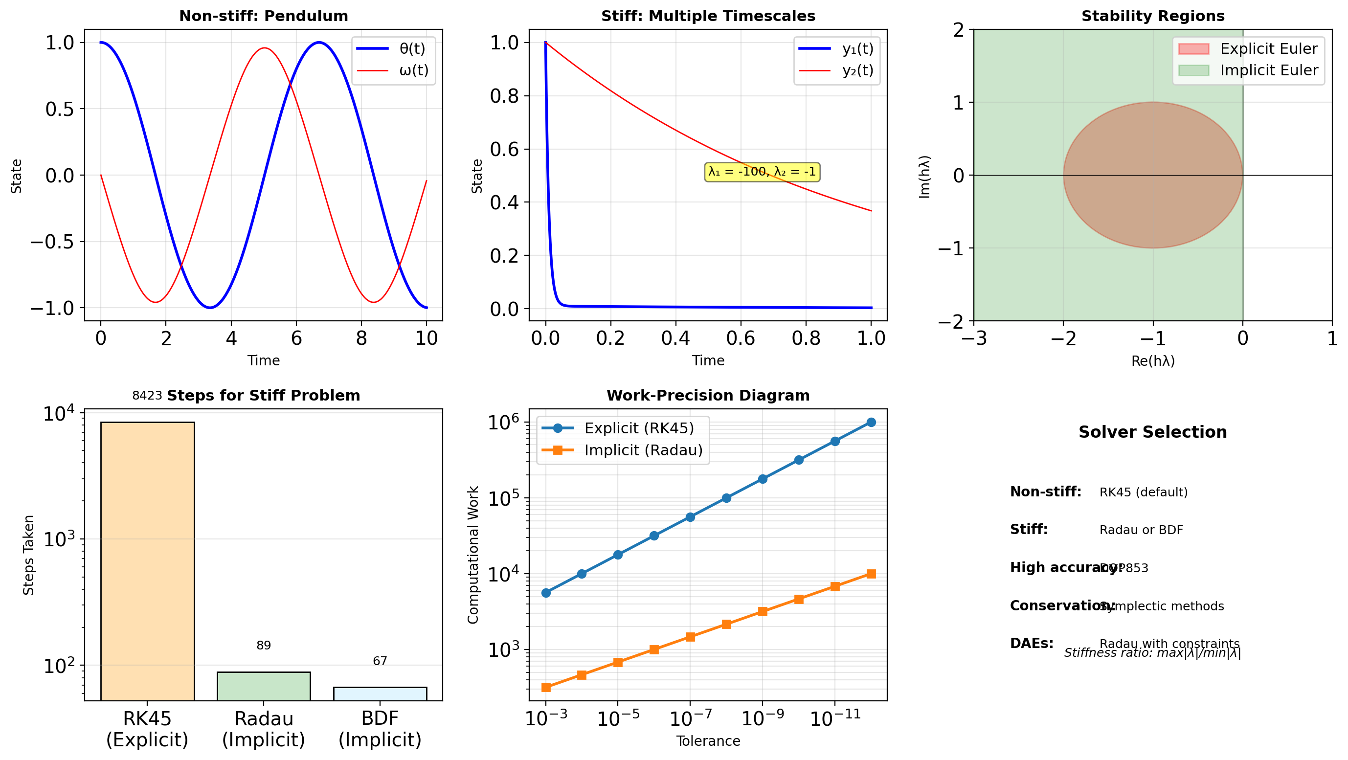
from functools import partial, reduce
import operator
# Partial function application
def power(base, exponent):
return base ** exponent
# Create specialized functions
square = partial(power, exponent=2)
cube = partial(power, exponent=3)
two_to_power = partial(power, base=2) # 2^x
print("Partial functions:")
print(f" square(5) = {square(5)}")
print(f" cube(5) = {cube(5)}")
print(f" 2^10 = {two_to_power(exponent=10)}")
# Partial with multiple arguments
def integrate(func, lower, upper, method='trapezoid', n_points=100):
"""Numerical integration."""
x = np.linspace(lower, upper, n_points)
y = func(x)
if method == 'trapezoid':
return np.trapezoid(y, x)
elif method == 'simpson':
from scipy.integrate import simpson
return simpson(y, x=x)
else:
raise ValueError(f"Unknown method: {method}")
# Create specialized integrators
simpson_integrate = partial(integrate, method='simpson')
unit_integrate = partial(integrate, lower=0, upper=1)
precise_integrate = partial(integrate, n_points=1000)
# Use specialized versions
result1 = simpson_integrate(np.sin, 0, np.pi)
result2 = unit_integrate(lambda x: x**2)
result3 = precise_integrate(np.exp, 0, 1)
print(f"\nIntegration results:")
print(f" ∫sin(x)dx [0,π] = {result1:.4f}")
print(f" ∫x²dx [0,1] = {result2:.4f}")
print(f" ∫e^x dx [0,1] = {result3:.4f}")Partial functions:
square(5) = 25
cube(5) = 125
2^10 = 1024
Integration results:
∫sin(x)dx [0,π] = 2.0000
∫x²dx [0,1] = 0.3334
∫e^x dx [0,1] = 1.7183functools.partial use cases:
- Pre-filling arguments for callbacks
- Creating specialized versions of general functions
- Configuration injection (default parameters)
# Common pattern: create specialized functions
from functools import partial
# Pre-configured logger
debug_log = partial(print, "[DEBUG]")
error_log = partial(print, "[ERROR]")
# Pre-configured numerical operations
normalize = partial(np.divide, b=255.0)
clip_unit = partial(np.clip, a_min=0, a_max=1)Currying (sequential application) is less common in Python than in functional languages. Use partial instead — it’s explicit and readable.
Composition pattern:
def compose(*funcs):
"""Compose functions: compose(f, g)(x) = f(g(x))"""
return reduce(lambda f, g: lambda x: f(g(x)), funcs)Decorators for Instrumentation
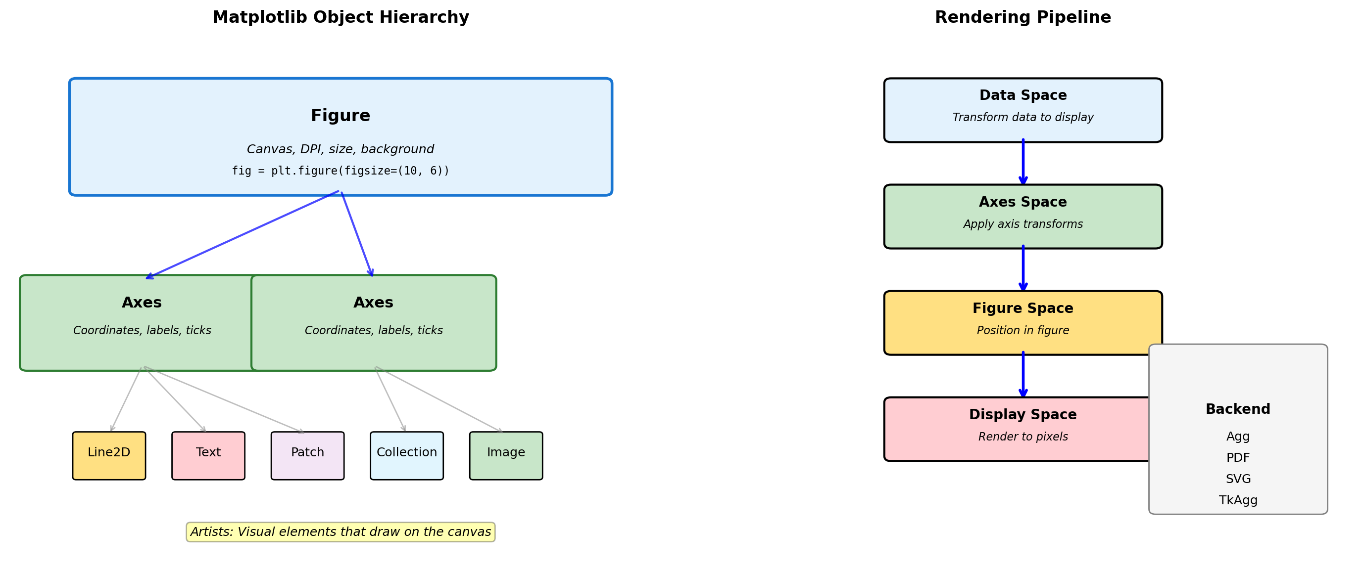
import time
import functools
def timer(func):
"""Simple timing decorator."""
@functools.wraps(func)
def wrapper(*args, **kwargs):
start = time.perf_counter()
result = func(*args, **kwargs)
elapsed = time.perf_counter() - start
print(f"{func.__name__} took {elapsed:.4f}s")
return result
return wrapper
@timer
def compute_sum(n):
"""Sum integers from 0 to n."""
return sum(range(n))
# Use decorated function
result = compute_sum(1000000)
print(f"Result: {result}")
# Decorator with arguments (decorator factory)
def repeat(n_times):
"""Decorator factory: repeat function call."""
def decorator(func):
@functools.wraps(func)
def wrapper(*args, **kwargs):
results = []
for _ in range(n_times):
results.append(func(*args, **kwargs))
return results
return wrapper
return decorator
@repeat(3)
def random_number():
import random
return random.random()
print(f"\nThree random numbers: {random_number()}")compute_sum took 0.0072s
Result: 499999500000
Three random numbers: [0.6994111129315287, 0.8404120796529236, 0.21618029945569128]Decorator pattern:
@decorator
def func():
pass
# Equivalent to:
func = decorator(func)Use functools.wraps to preserve the original function’s metadata (__name__, __doc__).
Common decorator uses:
- Timing/profiling
- Logging
- Caching (
@functools.lru_cache) - Validation
- Authentication/authorization
Decorator factory (decorator with arguments):
@factory(arg) # factory(arg) returns decorator
def func():
pass
# Equivalent to:
func = factory(arg)(func)Stacking decorators:
@dec1
@dec2
def func(): pass
# Equivalent to: func = dec1(dec2(func))
# dec2 wraps func first, then dec1 wraps thatSciPy Architecture: Python Interface to Fortran/C Libraries
SciPy provides Python bindings to decades of optimized numerical code.
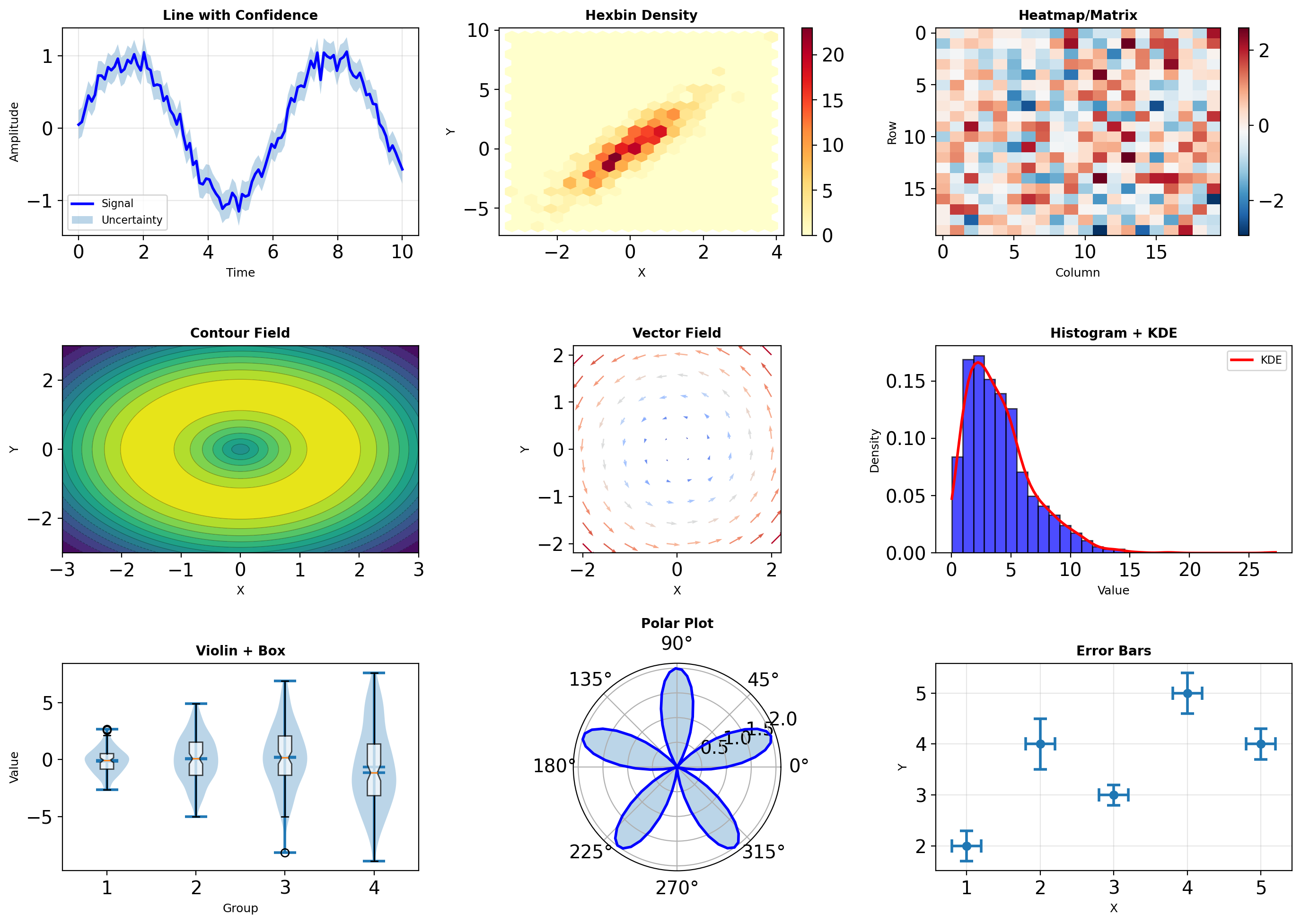
import scipy
import numpy as np
import timeit
# Demonstrate overhead vs computation
def small_operation():
"""Python function call dominates."""
A = np.array([[1, 2], [3, 4]])
return scipy.linalg.inv(A)
def large_operation():
"""Fortran computation dominates."""
A = np.random.randn(1000, 1000)
return scipy.linalg.inv(A)
# Measure call overhead
empty_call = timeit.timeit(lambda: None, number=100000)
print(f"Python function call: {empty_call*10:.2f}μs")
# Small vs large operation efficiency
A_small = np.random.randn(2, 2)
A_large = np.random.randn(100, 100)
t_small = timeit.timeit(
lambda: scipy.linalg.inv(A_small),
number=10000
)
t_large = timeit.timeit(
lambda: scipy.linalg.inv(A_large),
number=100
)
print(f"\n2×2 inversion: {t_small/10:.1f}μs per call")
print(f"100×100 inversion: {t_large*10:.1f}ms per call")
# BLAS level comparison
flops_small = 2**3 # O(n³) for inversion
flops_large = 100**3
print(f"\nFLOPS ratio: {flops_large/flops_small:,.0f}×")
print(f"Time ratio: {(t_large/100)/(t_small/10000):.0f}×")
print(f"Efficiency gain: {(flops_large/flops_small)/((t_large/100)/(t_small/10000)):.1f}×")Python function call: 0.01μs
2×2 inversion: 0.0μs per call
100×100 inversion: 0.1ms per call
FLOPS ratio: 125,000×
Time ratio: 49×
Efficiency gain: 2559.3×Design Implications:
Wrapper overhead is constant - Same Python call cost regardless of problem size
Amortization strategy - Process vectors/matrices, not scalars
Library selection hierarchy:
- Intel MKL (commercial, fastest)
- OpenBLAS (open source, competitive)
- Reference BLAS (portable, slow)
Memory layout matters - Fortran order (column-major) vs C order (row-major)
# SciPy provides optimized numerical routines
print(f"SciPy version: {scipy.__version__}")
print(f"Available submodules: {len([m for m in dir(scipy) if not m.startswith('_')])}")SciPy version: 1.17.1
Available submodules: 21Optimization: Interior Point vs Simplex Methods
Different algorithms excel at different problem structures.
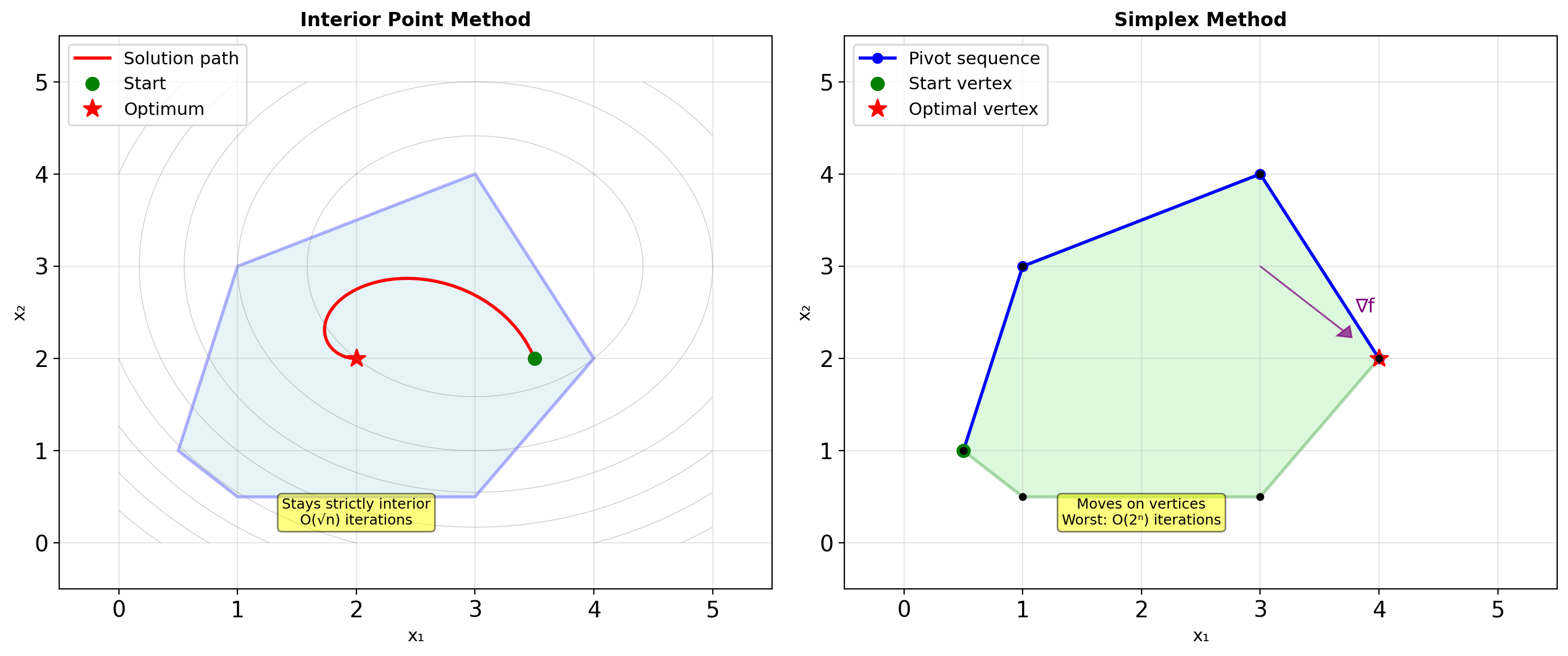
from scipy.optimize import linprog
import numpy as np
# Linear programming problem:
# minimize: -x - 2y
# subject to: x + 2y <= 8
# 2x + y <= 8
# x, y >= 0
c = [-1, -2] # Coefficients (minimize)
A_ub = [[1, 2], [2, 1]] # Inequality constraints
b_ub = [8, 8]
bounds = [(0, None), (0, None)]
# Compare methods
methods = ['interior-point', 'simplex', 'highs']
for method in methods:
result = linprog(c, A_ub=A_ub, b_ub=b_ub,
bounds=bounds, method=method)
print(f"{method:15s}: x={result.x}, "
f"iterations={result.nit}")
# Performance characteristics
n_vars = [10, 100, 1000]
for n in n_vars:
# Random LP problem
c = np.random.randn(n)
A = np.random.randn(n//2, n)
b = np.random.randn(n//2)
import time
# Interior point
start = time.perf_counter()
res_ip = linprog(c, A_ub=A, b_ub=b,
method='interior-point',
options={'disp': False})
time_ip = time.perf_counter() - start
# Simplex
start = time.perf_counter()
res_simplex = linprog(c, A_ub=A, b_ub=b,
method='simplex',
options={'disp': False})
time_simplex = time.perf_counter() - start
print(f"\nn={n:4d} variables:")
print(f" Interior: {time_ip*1000:6.1f}ms")
print(f" Simplex: {time_simplex*1000:6.1f}ms")interior-point : x=[1.69596234 3.15201883], iterations=4
simplex : x=[2.66666667 2.66666667], iterations=2
highs : x=[0. 4.], iterations=2
n= 10 variables:
Interior: 1.5ms
Simplex: 2.4ms
n= 100 variables:
Interior: 3.8ms
Simplex: 36.0ms
n=1000 variables:
Interior: 50.2ms
Simplex: 905.7msAlgorithm Selection Criteria:
Interior Point:
- Polynomial worst-case: O(n³·⁵)
- Better for large, dense problems
- Generates strictly feasible iterates
- Smooth convergence profile
Simplex:
- Exponential worst-case, excellent average-case
- Superior for sparse problems
- Always at a vertex (basic feasible solution)
- Can exploit problem structure
Modern hybrids (HiGHS):
- Crossover between methods
- Presolver eliminates variables
- Parallel execution paths
Root Finding: Convergence Rates and Stability
Root finding methods trade convergence speed for robustness.
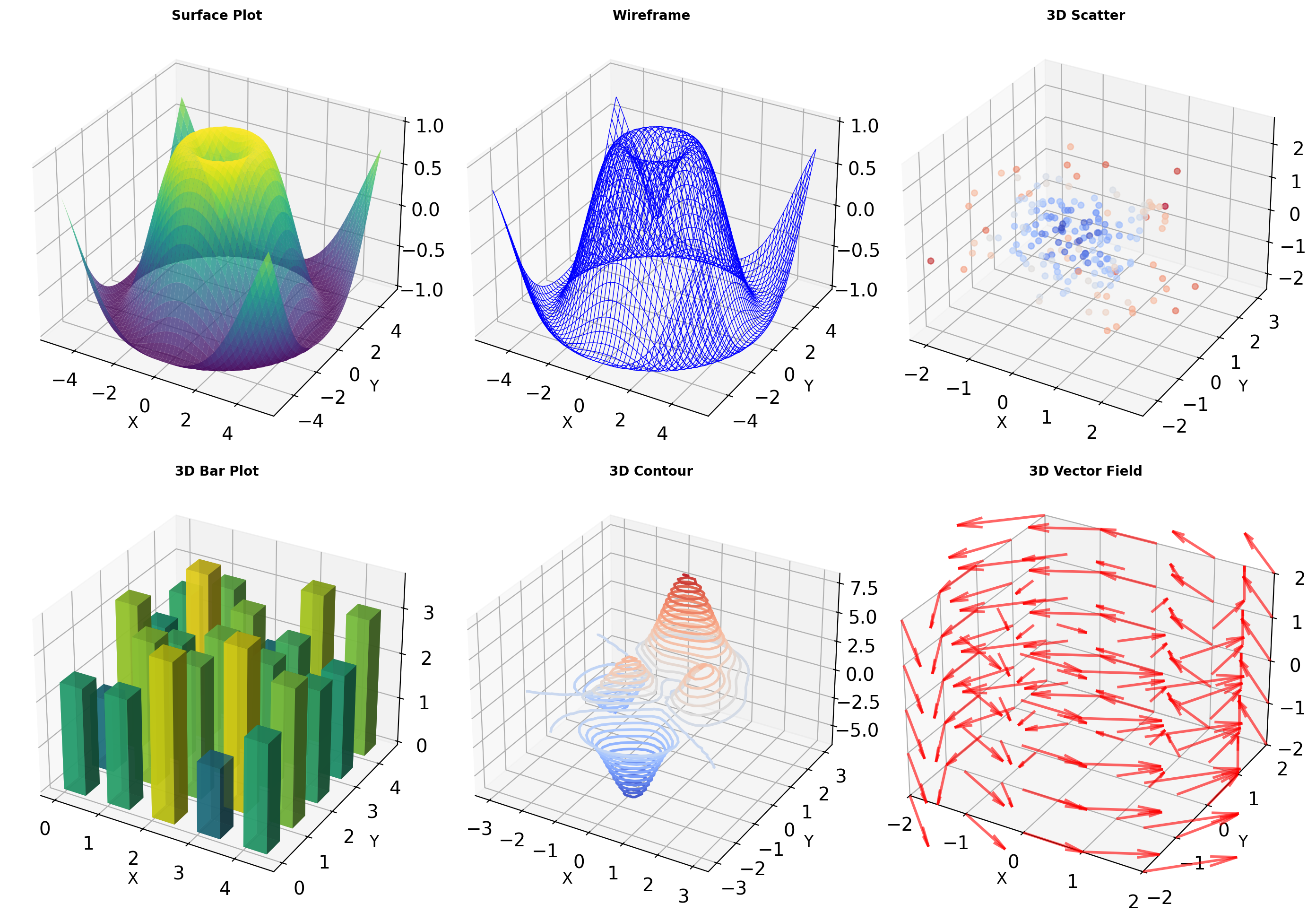
from scipy import optimize
import numpy as np
def f(x):
"""Test function with known root."""
return x**3 - x - 1
def fprime(x):
"""Derivative of f."""
return 3*x**2 - 1
# Compare root finding methods
x0 = 2.0 # Initial guess
bracket = [1, 2] # Known bracket
# Bisection: guaranteed convergence
root_bisect = optimize.bisect(f, *bracket)
print(f"Bisection: {root_bisect:.10f}")
# Brent: combines bisection, secant, inverse quadratic
root_brent = optimize.brentq(f, *bracket)
print(f"Brent: {root_brent:.10f}")
# Newton: fast but needs derivative
root_newton = optimize.newton(f, x0, fprime=fprime)
print(f"Newton: {root_newton:.10f}")
# Performance comparison
import timeit
n = 1000
times = {}
times['bisect'] = timeit.timeit(
lambda: optimize.bisect(f, 1, 2),
number=n
)
times['brent'] = timeit.timeit(
lambda: optimize.brentq(f, 1, 2),
number=n
)
times['newton'] = timeit.timeit(
lambda: optimize.newton(f, 2.0, fprime=fprime),
number=n
)
print(f"\nTime for {n} root findings:")
for method, time in times.items():
print(f" {method:8s}: {time*1000:.1f}ms")Bisection: 1.3247179572
Brent: 1.3247179572
Newton: 1.3247179572
Time for 1000 root findings:
bisect : 15.9ms
brent : 4.3ms
newton : 37.3msMethod Characteristics:
Bisection:
- Requires bracket [a, b] where f(a)·f(b) < 0
- Guaranteed convergence
- Linear rate: log₂(ε₀/ε) iterations
- One function evaluation per iteration
Newton-Raphson:
- Requires derivative
- Quadratic convergence near root
- Can diverge or cycle
- Two evaluations per iteration (f and f’)
Brent’s Method (scipy default):
- Hybrid: bisection + secant + inverse quadratic
- Guaranteed convergence with bracket
- Superlinear convergence in practice
- Adaptive algorithm selection
Numerical Integration: Adaptive Quadrature
Integration routines balance function evaluations against accuracy.
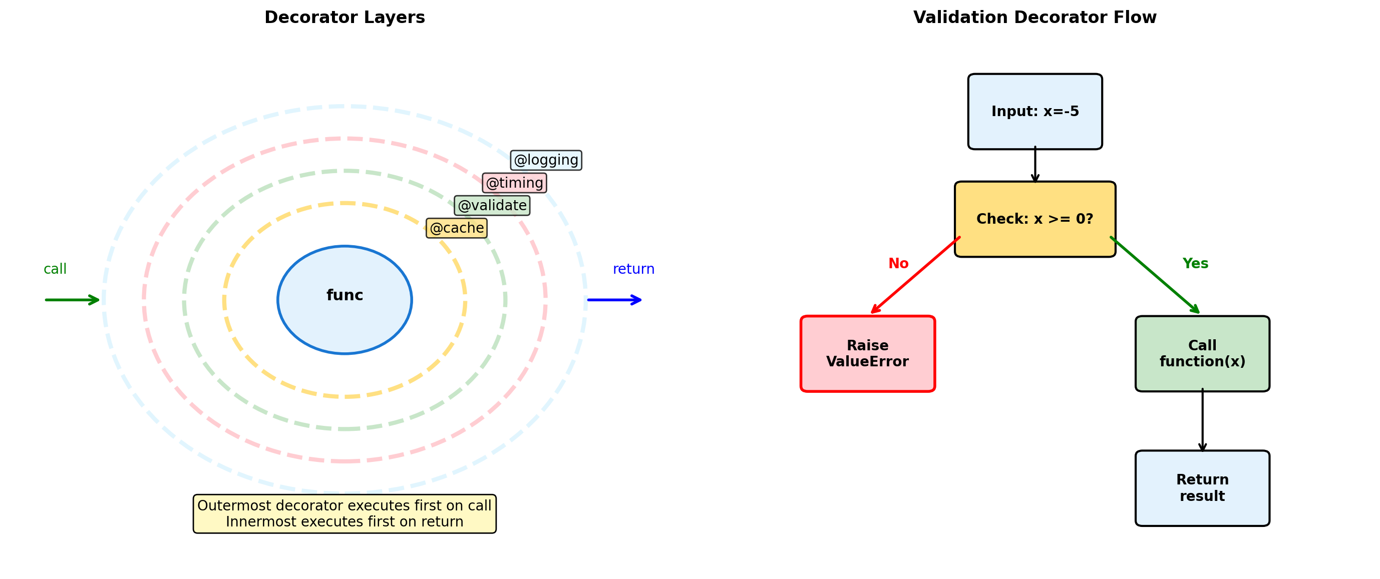
from scipy import integrate
import numpy as np
def oscillatory(x):
"""Challenging integrand."""
return np.exp(-x**2) * np.cos(10*x)
# Basic integration
result, error = integrate.quad(oscillatory, 0, 3)
print(f"quad result: {result:.8f} ± {error:.2e}")
# Show function evaluation count
full_output = integrate.quad(oscillatory, 0, 3,
full_output=True)
result, error, info = full_output
print(f"Function evaluations: {info['neval']}")
# Compare tolerances
tolerances = [1e-3, 1e-6, 1e-9]
for tol in tolerances:
result, error, info = integrate.quad(
oscillatory, 0, 3,
epsabs=tol, full_output=True
)
print(f"tol={tol:.0e}: {info['neval']:3d} evals, "
f"error={error:.2e}")
# Fixed vs adaptive sampling
def fixed_trapezoid(f, a, b, n):
"""Fixed spacing trapezoid rule."""
x = np.linspace(a, b, n)
y = f(x)
return np.trapezoid(y, x)
n_fixed = 1000
result_fixed = fixed_trapezoid(oscillatory, 0, 3, n_fixed)
result_adaptive, _, info = integrate.quad(
oscillatory, 0, 3, full_output=True
)
print(f"\nFixed {n_fixed} points: {result_fixed:.6f}")
print(f"Adaptive {info['neval']} points: {result_adaptive:.6f}")quad result: -0.00000982 ± 6.48e-15
Function evaluations: 147
tol=1e-03: 63 evals, error=4.38e-06
tol=1e-06: 105 evals, error=9.08e-08
tol=1e-09: 147 evals, error=6.48e-15
Fixed 1000 points: -0.000010
Adaptive 147 points: -0.000010QUADPACK Algorithms (scipy.integrate):
quad (adaptive quadrature):
- Gauss-Kronrod 21-point rule
- Error estimate from embedded 10-point rule
- Bisects intervals exceeding tolerance
- Globally adaptive strategy
Performance Factors:
- Smoothness: Higher derivatives → faster convergence
- Oscillations: Require subdivision
- Singularities: Special handling needed
- Dimensionality: Curse affects all methods
Specialized Routines:
quad_vec: Vectorized integrandsnquad: Multiple integrationdblquad,tplquad: 2D/3D convenienceodeint: ODE integration
Sparse Matrices: Storage Formats
Sparse matrices store only non-zero elements, trading format complexity for memory efficiency.

Format Selection
- COO: Best for construction and adding entries
- CSR: Best for row slicing and matrix-vector products
- CSC: Best for column slicing and linear solvers
import scipy.sparse as sp
import numpy as np
# Create sparse matrix
n = 1000
density = 0.01
A_dense = sp.rand(n, n, density=density, format='dense')
A_dense = np.array(A_dense)
# Convert to different formats
A_coo = sp.coo_matrix(A_dense)
A_csr = sp.csr_matrix(A_dense)
A_csc = sp.csc_matrix(A_dense)
# Memory usage
import sys
dense_size = sys.getsizeof(A_dense) / 1024**2
coo_size = (A_coo.data.nbytes +
A_coo.row.nbytes +
A_coo.col.nbytes) / 1024**2
csr_size = (A_csr.data.nbytes +
A_csr.indices.nbytes +
A_csr.indptr.nbytes) / 1024**2
print(f"Matrix {n}×{n}, density {density:.1%}")
print(f"Dense: {dense_size:.2f} MB")
print(f"COO: {coo_size:.2f} MB ({dense_size/coo_size:.1f}× smaller)")
print(f"CSR: {csr_size:.2f} MB ({dense_size/csr_size:.1f}× smaller)")
# Operation performance
v = np.random.randn(n)
import timeit
t_dense = timeit.timeit(lambda: A_dense @ v, number=100)
t_csr = timeit.timeit(lambda: A_csr @ v, number=100)
print(f"\nMatrix-vector multiply (100 iterations):")
print(f"Dense: {t_dense*1000:.1f}ms")
print(f"CSR: {t_csr*1000:.1f}ms ({t_dense/t_csr:.1f}× faster)")
# Format conversion cost
t_to_csr = timeit.timeit(
lambda: sp.csr_matrix(A_dense),
number=10
)
print(f"\nConversion to CSR: {t_to_csr*100:.1f}ms")Matrix 1000×1000, density 1.0%
Dense: 7.63 MB
COO: 0.15 MB (50.0× smaller)
CSR: 0.12 MB (64.5× smaller)
Matrix-vector multiply (100 iterations):
Dense: 1.6ms
CSR: 0.8ms (2.0× faster)
Conversion to CSR: 2.2msStorage Format Trade-offs:
COO (Coordinate):
- Three arrays: (row, col, data)
- No sorting required
- Allows duplicates (summed on conversion)
- Inefficient for arithmetic
CSR/CSC (Compressed Sparse Row/Column):
- Row-wise: (indptr, indices, data)
- Efficient row/column access
- Fast matrix-vector products
- Standard solver format
Performance Implications:
- Dense wins below ~10% density
- Format conversion has significant cost
- Row vs column access patterns matter
- In-place operations often impossible
Matplotlib Architecture: Object Hierarchy
Matplotlib uses a hierarchical object model that separates concerns across multiple abstraction levels.
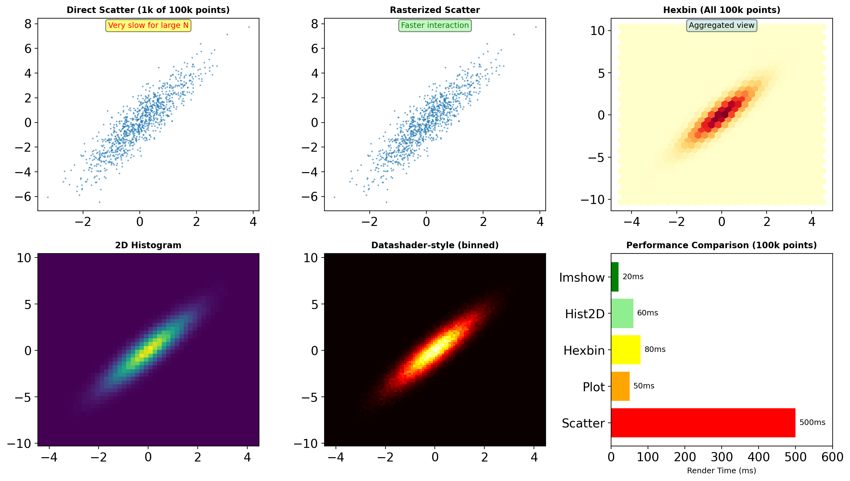
import matplotlib.pyplot as plt
import matplotlib as mpl
# Examine object hierarchy
fig = plt.figure(figsize=(8, 4))
ax1 = fig.add_subplot(121)
ax2 = fig.add_subplot(122)
# Plot creates multiple artists
line, = ax1.plot([1, 2, 3], [1, 4, 2], 'b-')
scatter = ax2.scatter([1, 2, 3], [2, 3, 1])
# Object relationships
print("Figure attributes:")
print(f" Number of axes: {len(fig.axes)}")
print(f" DPI: {fig.dpi}")
print(f" Size: {fig.get_size_inches()} inches")
print("\nAxes ax1 contents:")
print(f" Lines: {len(ax1.lines)}")
print(f" Patches: {len(ax1.patches)}")
print(f" Texts: {len(ax1.texts)}")
print(f" Artists: {len(ax1.get_children())}")
# Access artist properties
print(f"\nLine2D properties:")
print(f" Data: x={line.get_xdata()}, y={line.get_ydata()}")
print(f" Color: {line.get_color()}")
print(f" Linewidth: {line.get_linewidth()}")
print(f" Marker: '{line.get_marker()}'")
# Transform pipeline
data_point = (2, 4)
display_point = ax1.transData.transform(data_point)
figure_point = fig.transFigure.inverted().transform(display_point)
print(f"\nTransform pipeline for {data_point}:")
print(f" Data space: {data_point}")
print(f" Display space: {display_point}")
print(f" Figure space: {figure_point}")
plt.close() # Clean upFigure attributes:
Number of axes: 2
DPI: 100.0
Size: [8. 4.] inches
Axes ax1 contents:
Lines: 1
Patches: 0
Texts: 0
Artists: 11
Line2D properties:
Data: x=[1 2 3], y=[1 4 2]
Color: b
Linewidth: 2.0
Marker: 'None'
Transform pipeline for (2, 4):
Data space: (2, 4)
Display space: [ 663.63636364 1276. ]
Figure space: [0.82954545 3.19 ]Architecture Components:
Figure: Top-level container
- Manages canvas and renderer
- Controls output size and DPI
- Contains one or more Axes
Axes: Plotting area with coordinates
- Data limits and scaling
- Tick locators and formatters
- Contains Artists
Artists: Everything visible
- Primitives: Line2D, Rectangle, Text
- Collections: LineCollection, PathCollection
- Containers: Axis, Legend
Transforms: Coordinate mappings
- Data → Axes → Figure → Display
- Enables zoom, pan, aspect ratio
Backend: Rendering engine
- Interactive: Qt5Agg, TkAgg
- Hardcopy: Agg, PDF, SVG
Plot Types for Scientific Data
Different visualizations optimize for different data characteristics and analysis goals.

import matplotlib.pyplot as plt
import numpy as np
# Performance comparison for different plot types
data_sizes = [100, 1000, 10000, 100000]
plot_types = {
'line': lambda ax, n: ax.plot(np.arange(n), np.random.randn(n)),
'scatter': lambda ax, n: ax.scatter(np.arange(n), np.random.randn(n)),
'hist': lambda ax, n: ax.hist(np.random.randn(n), bins=50),
'imshow': lambda ax, n: ax.imshow(np.random.randn(int(np.sqrt(n)), int(np.sqrt(n)))),
}
import time
print("Rendering time (ms) for different plot types:")
print(f"{'Size':<10} {'Line':<10} {'Scatter':<10} {'Hist':<10} {'Imshow':<10}")
print("-" * 50)
for size in data_sizes:
times = {}
for plot_type, plot_func in plot_types.items():
fig, ax = plt.subplots()
start = time.perf_counter()
plot_func(ax, size)
fig.canvas.draw()
elapsed = (time.perf_counter() - start) * 1000
times[plot_type] = elapsed
plt.close(fig)
print(f"{size:<10} {times['line']:<10.1f} {times['scatter']:<10.1f} "
f"{times['hist']:<10.1f} {times['imshow']:<10.1f}")
# Memory usage analysis
import sys
fig, ax = plt.subplots()
line, = ax.plot(np.arange(10000), np.random.randn(10000))
scatter = ax.scatter(np.arange(1000), np.random.randn(1000))
print(f"\nMemory usage:")
print(f" Line (10k points): ~{sys.getsizeof(line.get_xydata()) / 1024:.1f} KB")
print(f" Scatter (1k points): ~{sys.getsizeof(scatter.get_offsets()) / 1024:.1f} KB")
plt.close()Rendering time (ms) for different plot types:
Size Line Scatter Hist Imshow
--------------------------------------------------
100 9.0 8.1 123.1 11.7
1000 13.6 8.8 15.3 13.3
10000 60.2 12.3 16.7 11.3
100000 284.1 41.6 17.3 18.8
Memory usage:
Line (10k points): ~156.4 KB
Scatter (1k points): ~0.2 KBPlot Selection Criteria:
Continuous Data:
- Line: Time series, functions
- Fill: Confidence intervals, ranges
- Contour: 2D scalar fields
Discrete Points:
- Scatter: Correlations, outliers
- Hexbin: Large datasets (>10k points)
- Histogram: Distributions
Statistical:
- Box: Quartiles and outliers
- Violin: Distribution shape
- Error bars: Measurement uncertainty
Performance Tips:
- Use
plot()overscatter()for large datasets - Rasterize dense plots:
rasterized=True - Downsample data before plotting
- Use blitting for animations
Subplot Layouts and Composition
Complex figures require careful layout management for effective visualization.
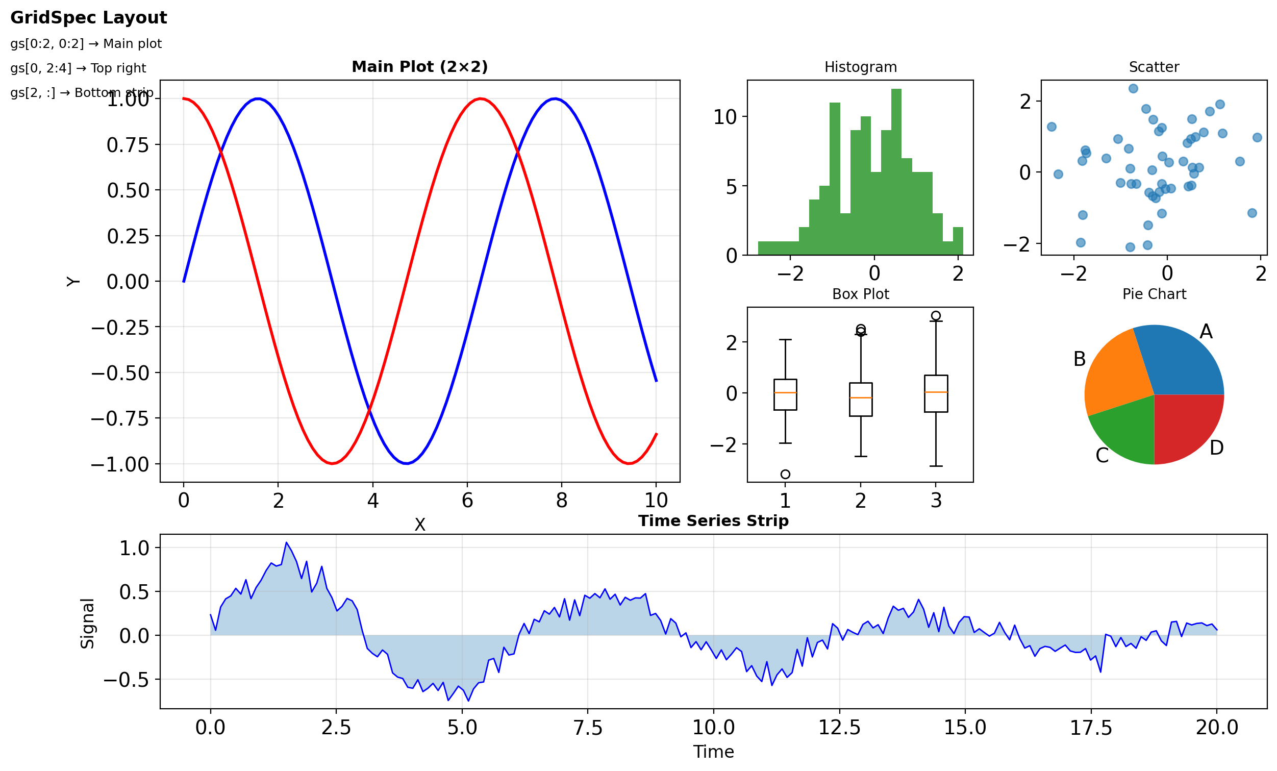
import matplotlib.pyplot as plt
import matplotlib.gridspec as gridspec
import numpy as np
# Method 1: Simple grid
fig1, axes = plt.subplots(2, 3, figsize=(9, 6))
print(f"Simple grid: {axes.shape} axes")
# Method 2: GridSpec for complex layouts
fig2 = plt.figure(figsize=(10, 6))
gs = gridspec.GridSpec(3, 3, figure=fig2,
width_ratios=[1, 2, 1],
height_ratios=[1, 2, 1],
hspace=0.3, wspace=0.3)
# Create axes with different spans
ax1 = fig2.add_subplot(gs[0, :]) # Top row, all columns
ax2 = fig2.add_subplot(gs[1:, 0]) # Rows 1-2, first column
ax3 = fig2.add_subplot(gs[1:, 1:]) # Rows 1-2, columns 1-2
print(f"\nGridSpec axes positions:")
print(f" ax1: {ax1.get_position()}")
print(f" ax2: {ax2.get_position()}")
print(f" ax3: {ax3.get_position()}")
# Method 3: Nested layouts
fig3 = plt.figure(figsize=(10, 6))
outer_grid = gridspec.GridSpec(2, 2, figure=fig3)
# Nested grid in first cell
inner_grid = gridspec.GridSpecFromSubplotSpec(
2, 2, subplot_spec=outer_grid[0, 0]
)
# Create nested axes
for i in range(2):
for j in range(2):
ax = fig3.add_subplot(inner_grid[i, j])
ax.text(0.5, 0.5, f'({i},{j})', ha='center')
# Regular axes in other cells
ax_right = fig3.add_subplot(outer_grid[0, 1])
ax_bottom = fig3.add_subplot(outer_grid[1, :])
plt.close('all') # Clean up
# Constrained layout for automatic spacing
fig4, axes = plt.subplots(2, 2, figsize=(8, 6),
constrained_layout=True)
for ax in axes.flat:
ax.plot(np.random.randn(100))
ax.set_title('Auto-spaced')
print("\nConstrained layout automatically adjusts spacing")
plt.close('all')Simple grid: (2, 3) axes
GridSpec axes positions:
ax1: Bbox(x0=0.125, y0=0.7195833333333334, x1=0.9000000000000001, y1=0.88)
ax2: Bbox(x0=0.125, y0=0.10999999999999999, x1=0.28645833333333337, y1=0.6554166666666668)
ax3: Bbox(x0=0.3510416666666667, y0=0.10999999999999999, x1=0.9000000000000001, y1=0.6554166666666668)
Constrained layout automatically adjusts spacing# Shared axes for comparison
fig, axes = plt.subplots(3, 1, figsize=(8, 6),
sharex=True)
x = np.linspace(0, 10, 100)
data = [np.sin(x), np.cos(x), np.sin(x) * np.cos(x)]
labels = ['sin(x)', 'cos(x)', 'sin(x)cos(x)']
for ax, y, label in zip(axes, data, labels):
ax.plot(x, y, linewidth=2)
ax.set_ylabel(label)
ax.grid(True, alpha=0.3)
# Only bottom axis shows x-label
if ax == axes[-1]:
ax.set_xlabel('X')
axes[0].set_title('Shared X-axis', fontweight='bold')
# Measure rendering overhead
import time
layout_times = {}
# Simple layout
start = time.perf_counter()
fig, axes = plt.subplots(3, 3)
fig.canvas.draw()
layout_times['simple'] = time.perf_counter() - start
# Complex GridSpec
start = time.perf_counter()
fig = plt.figure()
gs = gridspec.GridSpec(5, 5)
for i in range(5):
for j in range(5):
ax = fig.add_subplot(gs[i, j])
fig.canvas.draw()
layout_times['complex'] = time.perf_counter() - start
print("\nLayout creation overhead:")
for layout, t in layout_times.items():
print(f" {layout}: {t*1000:.1f}ms")
plt.close('all')
Layout creation overhead:
simple: 60.5ms
complex: 111.5ms3D Visualization
Three-dimensional plots require special consideration for perspective and interaction.
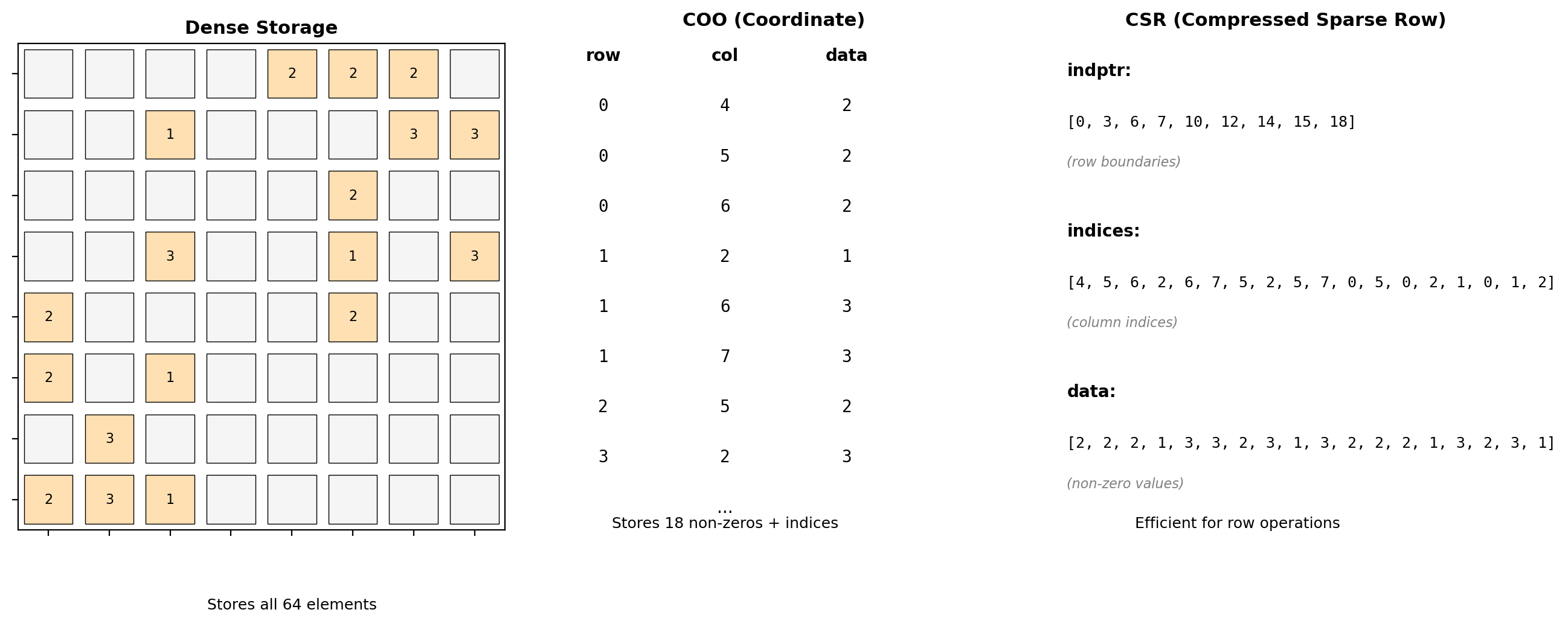
from mpl_toolkits.mplot3d import Axes3D
import numpy as np
import time
# Performance analysis for 3D plots
fig = plt.figure(figsize=(10, 5))
# Compare 2D vs 3D rendering
grid_sizes = [10, 20, 30, 40, 50]
times_2d = []
times_3d = []
for size in grid_sizes:
X = np.linspace(-5, 5, size)
Y = np.linspace(-5, 5, size)
X, Y = np.meshgrid(X, Y)
Z = np.sin(np.sqrt(X**2 + Y**2))
# 2D heatmap
fig2d, ax2d = plt.subplots()
start = time.perf_counter()
ax2d.imshow(Z)
fig2d.canvas.draw()
times_2d.append(time.perf_counter() - start)
plt.close(fig2d)
# 3D surface
fig3d = plt.figure()
ax3d = fig3d.add_subplot(111, projection='3d')
start = time.perf_counter()
ax3d.plot_surface(X, Y, Z)
fig3d.canvas.draw()
times_3d.append(time.perf_counter() - start)
plt.close(fig3d)
print("Rendering time comparison (ms):")
print(f"{'Grid':<10} {'2D Heatmap':<15} {'3D Surface':<15} {'Ratio':<10}")
print("-" * 50)
for i, size in enumerate(grid_sizes):
ratio = times_3d[i] / times_2d[i]
print(f"{size}×{size:<6} {times_2d[i]*1000:<15.1f} "
f"{times_3d[i]*1000:<15.1f} {ratio:<10.1f}x")
# View angle impact
fig = plt.figure()
ax = fig.add_subplot(111, projection='3d')
# Create surface
X = np.linspace(-5, 5, 30)
Y = np.linspace(-5, 5, 30)
X, Y = np.meshgrid(X, Y)
Z = np.sin(np.sqrt(X**2 + Y**2))
ax.plot_surface(X, Y, Z, cmap='viridis')
# Get view angles
elev = ax.elev
azim = ax.azim
print(f"\nDefault view angles:")
print(f" Elevation: {elev}°")
print(f" Azimuth: {azim}°")
# Programmatic rotation
ax.view_init(elev=30, azim=45)
print(f"Modified view: elev=30°, azim=45°")
plt.close()Rendering time comparison (ms):
Grid 2D Heatmap 3D Surface Ratio
--------------------------------------------------
10×10 12.0 14.1 1.2 x
20×20 14.2 21.0 1.5 x
30×30 12.4 27.6 2.2 x
40×40 13.5 40.1 3.0 x
50×50 11.4 54.6 4.8 x
Default view angles:
Elevation: 30°
Azimuth: -60°
Modified view: elev=30°, azim=45°<Figure size 1000x500 with 0 Axes># 3D plotting optimizations
import matplotlib.pyplot as plt
from mpl_toolkits.mplot3d import Axes3D
import numpy as np
# Optimization strategies
fig = plt.figure(figsize=(8, 4))
# Strategy 1: Reduce resolution
ax1 = fig.add_subplot(121, projection='3d')
X_low = np.linspace(-5, 5, 20) # Low resolution
Y_low = np.linspace(-5, 5, 20)
X_low, Y_low = np.meshgrid(X_low, Y_low)
Z_low = np.sin(np.sqrt(X_low**2 + Y_low**2))
ax1.plot_surface(X_low, Y_low, Z_low,
cmap='viridis', alpha=0.8)
ax1.set_title('Low Resolution (Fast)')
# Strategy 2: Use simpler representations
ax2 = fig.add_subplot(122, projection='3d')
ax2.plot_wireframe(X_low, Y_low, Z_low,
color='blue', linewidth=0.5,
rstride=2, cstride=2) # Skip points
ax2.set_title('Wireframe (Faster)')
# Memory usage
import sys
surf_artist = ax1.collections[0]
wire_artist = ax2.collections[0]
print("\nMemory comparison:")
print(f" Surface plot: ~{len(surf_artist._facecolors)*4/1024:.1f} KB")
print(f" Wireframe: ~{len(wire_artist._segments3d)*24/1024:.1f} KB")
# Z-order sorting overhead
n_triangles = X_low.size * 2 # Approximate
print(f"\nZ-buffer sorting:")
print(f" Triangles to sort: ~{n_triangles}")
print(f" Complexity: O(n log n) = O({n_triangles} log {n_triangles})")
plt.tight_layout()
plt.close()
# Interactive considerations
print("\n3D interaction overhead:")
print(" Mouse rotation: Recomputes projections")
print(" Zoom: Recalculates clipping")
print(" Pan: Updates transform matrices")
Memory comparison:
Surface plot: ~0.0 KB
Wireframe: ~0.5 KB
Z-buffer sorting:
Triangles to sort: ~800
Complexity: O(n log n) = O(800 log 800)
3D interaction overhead:
Mouse rotation: Recomputes projections
Zoom: Recalculates clipping
Pan: Updates transform matricesAnimations for Time Series
Animations visualize temporal evolution but require careful performance optimization.
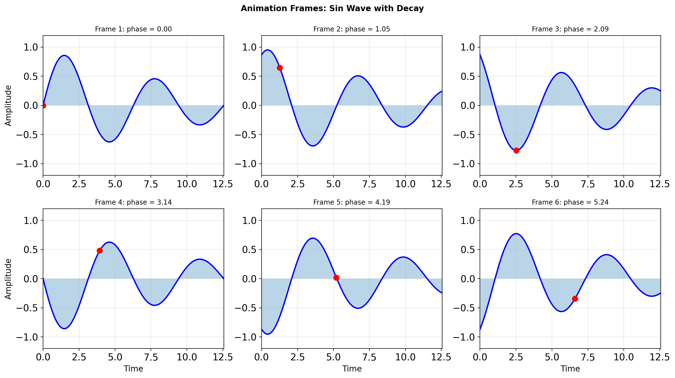
import matplotlib.pyplot as plt
import matplotlib.animation as animation
import numpy as np
# Basic animation structure
fig, (ax1, ax2) = plt.subplots(2, 1, figsize=(8, 6))
# Data setup
x = np.linspace(0, 2*np.pi, 100)
line1, = ax1.plot([], [], 'b-', linewidth=2)
line2, = ax2.plot([], [], 'r-', linewidth=2)
ax1.set_xlim(0, 2*np.pi)
ax1.set_ylim(-1.5, 1.5)
ax1.set_title('Animation with Blitting')
ax1.grid(True, alpha=0.3)
ax2.set_xlim(0, 2*np.pi)
ax2.set_ylim(-1.5, 1.5)
ax2.set_title('Accumulated History')
ax2.grid(True, alpha=0.3)
# Animation state
history = []
def init():
"""Initialize animation."""
line1.set_data([], [])
line2.set_data([], [])
return line1, line2
def animate(frame):
"""Animation function called for each frame."""
# Update data
y1 = np.sin(x + frame * 0.1)
line1.set_data(x, y1)
# Accumulate history
if len(history) > 50:
history.pop(0)
history.append(np.sin(2*np.pi * frame / 50))
# Plot history
if history:
line2.set_data(np.linspace(0, 2*np.pi, len(history)),
history)
return line1, line2
# Performance comparison
import time
# Without blitting
start = time.perf_counter()
for i in range(50):
animate(i)
fig.canvas.draw()
no_blit_time = time.perf_counter() - start
print(f"Animation performance (50 frames):")
print(f" Without blitting: {no_blit_time*1000:.1f}ms")
print(f" FPS: {50/no_blit_time:.1f}")
# Memory management
print(f"\nMemory considerations:")
print(f" Line data: {x.nbytes + x.nbytes} bytes per frame")
print(f" History buffer: {len(history) * 8} bytes")
print(f" Canvas cache: ~{fig.canvas.get_width_height()[0] * fig.canvas.get_width_height()[1] * 4} bytes")
plt.close()
# Optimization techniques
print("\nOptimization strategies:")
print(" 1. Use blitting: ~5-10x speedup")
print(" 2. Update only changed artists")
print(" 3. Reduce figure DPI for preview")
print(" 4. Cache static elements")
print(" 5. Use collections for many objects")Animation performance (50 frames):
Without blitting: 415.1ms
FPS: 120.5
Memory considerations:
Line data: 1600 bytes per frame
History buffer: 400 bytes
Canvas cache: ~1920000 bytes
Optimization strategies:
1. Use blitting: ~5-10x speedup
2. Update only changed artists
3. Reduce figure DPI for preview
4. Cache static elements
5. Use collections for many objectsAnimation structure:
# Create figure and line artist
fig, ax = plt.subplots()
line, = ax.plot([], [])
def init():
"""Set up blank frame."""
line.set_data([], [])
return line,
def animate(frame):
"""Update for each frame."""
y = np.sin(x + frame * 0.1)
line.set_data(x, y)
return line,
# Create animation
anim = FuncAnimation(fig, animate, init_func=init,
frames=100, interval=50, blit=True)
# Save to file
anim.save('animation.mp4', writer='ffmpeg', fps=30)Blitting caches the static background and redraws only the changed artists — typically 5-10x faster than full redraws.
blit=True requires:
init()andanimate()return iterables of updated artists- Artists must be on the same axes
- Background must not change between frames
Saving animations:
- MP4:
writer='ffmpeg'(requires ffmpeg installed) - GIF:
writer='pillow' - HTML5:
anim.to_jshtml()for notebooks
Performance Optimization for Large Datasets
Visualizing large datasets requires strategic optimization to maintain interactivity.
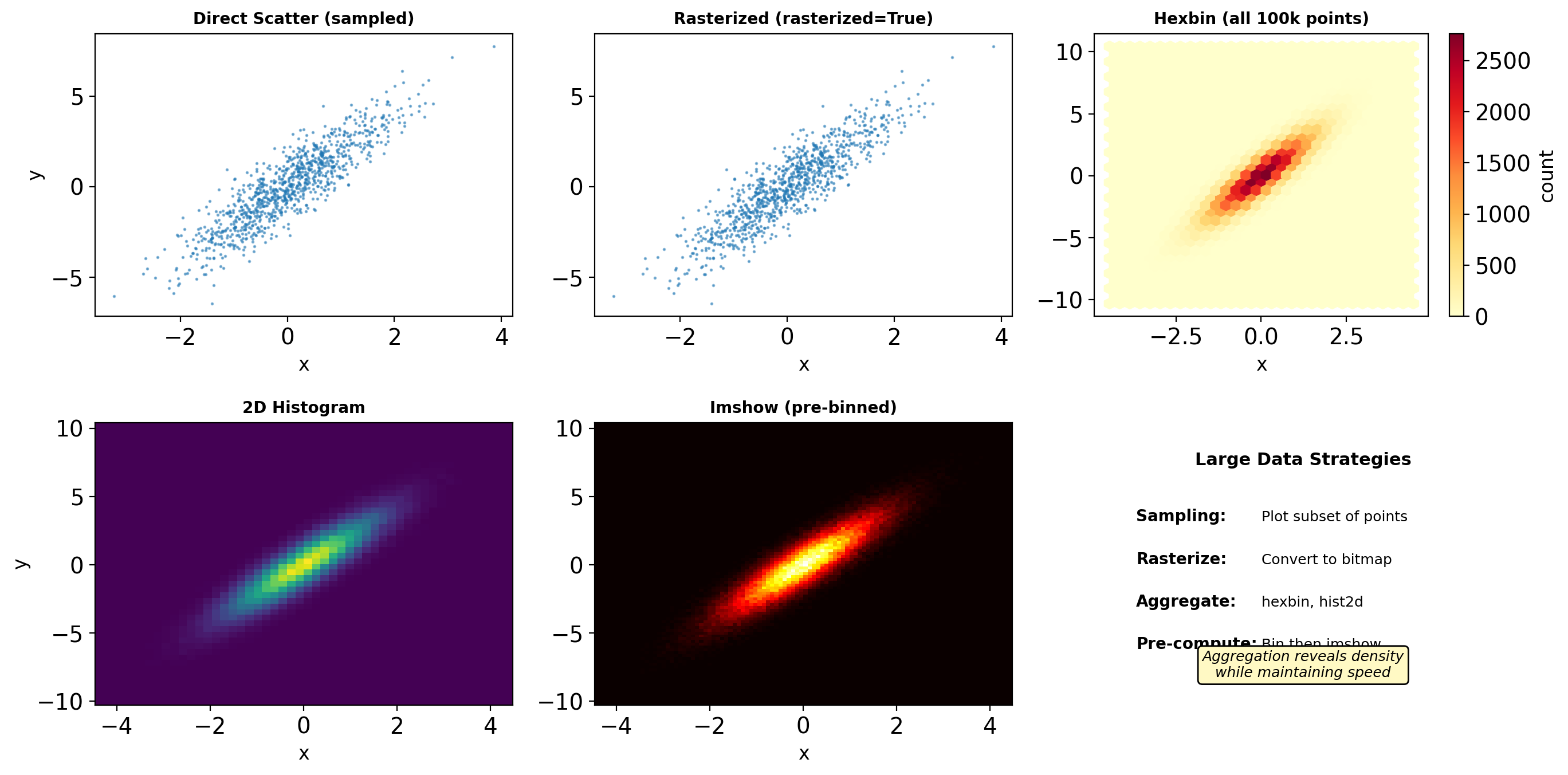
import matplotlib.pyplot as plt
import numpy as np
import time
# Generate large dataset
n_points = 50000
x = np.random.randn(n_points)
y = 2*x + np.random.randn(n_points)
# Benchmark different approaches
results = {}
# 1. Direct scatter (limited to 5k for speed)
fig, ax = plt.subplots()
start = time.perf_counter()
ax.scatter(x[:5000], y[:5000], alpha=0.5, s=1)
fig.canvas.draw()
results['scatter_5k'] = time.perf_counter() - start
plt.close()
# 2. Plot instead of scatter
fig, ax = plt.subplots()
start = time.perf_counter()
ax.plot(x, y, 'o', markersize=1, alpha=0.5)
fig.canvas.draw()
results['plot_50k'] = time.perf_counter() - start
plt.close()
# 3. Hexbin
fig, ax = plt.subplots()
start = time.perf_counter()
ax.hexbin(x, y, gridsize=30)
fig.canvas.draw()
results['hexbin_50k'] = time.perf_counter() - start
plt.close()
# 4. 2D histogram
fig, ax = plt.subplots()
start = time.perf_counter()
ax.hist2d(x, y, bins=50)
fig.canvas.draw()
results['hist2d_50k'] = time.perf_counter() - start
plt.close()
print("Rendering performance:")
for method, time_val in results.items():
print(f" {method:15s}: {time_val*1000:6.1f}ms")
# Memory usage estimation
import sys
# Scatter artist memory
fig, ax = plt.subplots()
scatter = ax.scatter(x[:1000], y[:1000])
scatter_memory = (sys.getsizeof(scatter.get_offsets()) +
sys.getsizeof(scatter.get_facecolors()))
# Line artist memory
line, = ax.plot(x[:1000], y[:1000], 'o')
line_memory = sys.getsizeof(line.get_xydata())
print(f"\nMemory usage (1000 points):")
print(f" Scatter: ~{scatter_memory/1024:.1f} KB")
print(f" Line: ~{line_memory/1024:.1f} KB")
print(f" Ratio: {scatter_memory/line_memory:.1f}x")
plt.close('all')Rendering performance:
scatter_5k : 11.9ms
plot_50k : 13.1ms
hexbin_50k : 17.9ms
hist2d_50k : 13.1ms
Memory usage (1000 points):
Scatter: ~0.3 KB
Line: ~15.8 KB
Ratio: 0.0x# Optimization strategies
class OptimizedPlotter:
"""Strategies for large dataset visualization."""
@staticmethod
def downsample(x, y, max_points=1000):
"""Randomly sample if too many points."""
n = len(x)
if n <= max_points:
return x, y
idx = np.random.choice(n, max_points, replace=False)
return x[idx], y[idx]
@staticmethod
def use_rasterization(ax, x, y):
"""Rasterize dense plots."""
ax.scatter(x, y, alpha=0.5, s=1, rasterized=True)
# Rasterized elements become bitmaps
# Faster zooming/panning
@staticmethod
def aggregate_data(x, y, bins=50):
"""Convert to density representation."""
H, xedges, yedges = np.histogram2d(x, y, bins=bins)
return H, xedges, yedges
@staticmethod
def progressive_rendering(x, y, ax):
"""Render in stages for responsiveness."""
# Quick preview
x_preview, y_preview = OptimizedPlotter.downsample(
x, y, max_points=100
)
line = ax.plot(x_preview, y_preview, 'o',
markersize=2, alpha=0.3)[0]
ax.figure.canvas.draw()
# Full render
line.set_data(x, y)
ax.figure.canvas.draw()
# Level-of-detail (LOD) system
class LODPlot:
"""Adaptive detail based on zoom level."""
def __init__(self, x, y):
self.x_full = x
self.y_full = y
self.create_levels()
def create_levels(self):
"""Create multiple resolution levels."""
self.levels = {}
n = len(self.x_full)
# Full resolution
self.levels[0] = (self.x_full, self.y_full)
# Reduced resolutions
for level in [1, 2, 3]:
step = 2 ** level
self.levels[level] = (
self.x_full[::step],
self.y_full[::step]
)
def get_data(self, zoom_level):
"""Return appropriate resolution."""
if zoom_level > 10:
return self.levels[0] # Full
elif zoom_level > 5:
return self.levels[1] # Half
elif zoom_level > 2:
return self.levels[2] # Quarter
else:
return self.levels[3] # Eighth
# Test LOD system
lod = LODPlot(x, y)
print("\nLOD system points at each level:")
for level in range(4):
x_level, y_level = lod.levels[level]
print(f" Level {level}: {len(x_level)} points")
# Chunked rendering for streaming
def chunked_plot(x, y, ax, chunk_size=5000):
"""Plot data in chunks to maintain responsiveness."""
n_chunks = len(x) // chunk_size + 1
for i in range(n_chunks):
start = i * chunk_size
end = min((i + 1) * chunk_size, len(x))
ax.plot(x[start:end], y[start:end], 'o',
markersize=1, alpha=0.5)
# Allow GUI to update
if i % 5 == 0:
ax.figure.canvas.draw()
plt.pause(0.001)
print("\nOptimization impact:")
print(" Rasterization: 2-5x faster interaction")
print(" Aggregation: 10-100x data reduction")
print(" LOD: Adaptive performance")
LOD system points at each level:
Level 0: 50000 points
Level 1: 25000 points
Level 2: 12500 points
Level 3: 6250 points
Optimization impact:
Rasterization: 2-5x faster interaction
Aggregation: 10-100x data reduction
LOD: Adaptive performanceBackend Selection and Output Formats
Different backends optimize for different use cases: interactivity vs. publication quality.
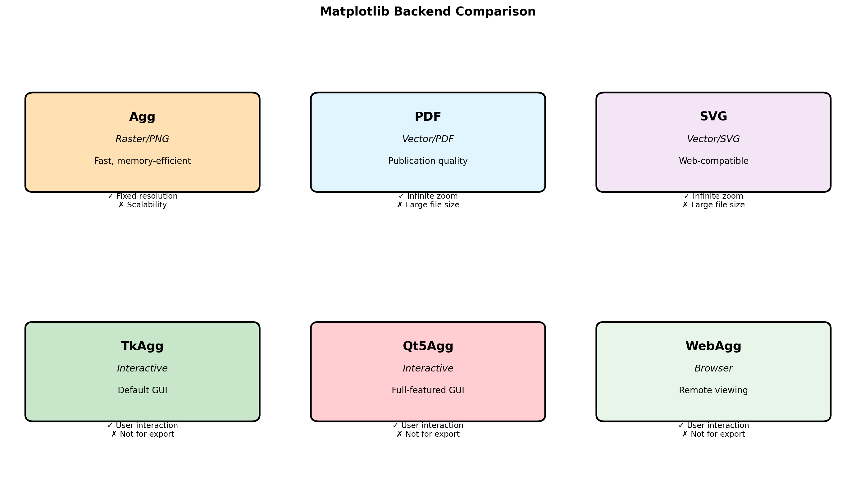
import matplotlib
import matplotlib.pyplot as plt
import numpy as np
import os
# Check available backends
print("Available backends:")
for backend in matplotlib.rcsetup.all_backends:
print(f" {backend}")
print(f"\nCurrent backend: {matplotlib.get_backend()}")
# Create test figure
fig, ax = plt.subplots(figsize=(6, 4))
x = np.linspace(0, 10, 1000)
ax.plot(x, np.sin(x), 'b-', linewidth=2)
ax.fill_between(x, 0, np.sin(x), alpha=0.3)
ax.set_title('Test Figure')
ax.grid(True, alpha=0.3)
# Save in different formats
formats = {
'png': {'dpi': 100, 'bbox_inches': 'tight'},
'pdf': {'bbox_inches': 'tight'},
'svg': {'bbox_inches': 'tight'},
'eps': {'bbox_inches': 'tight'},
}
file_sizes = {}
import time
for fmt, kwargs in formats.items():
filename = f'test_figure.{fmt}'
start = time.perf_counter()
fig.savefig(filename, format=fmt, **kwargs)
save_time = time.perf_counter() - start
# Check file size
if os.path.exists(filename):
size = os.path.getsize(filename) / 1024 # KB
file_sizes[fmt] = (size, save_time)
os.remove(filename) # Clean up
print("\nOutput format comparison:")
print(f"{'Format':<10} {'Size (KB)':<12} {'Time (ms)':<10}")
print("-" * 35)
for fmt, (size, save_time) in file_sizes.items():
print(f"{fmt:<10} {size:<12.1f} {save_time*1000:<10.1f}")
plt.close()
# DPI impact on file size
dpis = [72, 100, 150, 200, 300]
sizes = []
times = []
for dpi in dpis:
start = time.perf_counter()
fig.savefig('temp.png', dpi=dpi)
times.append(time.perf_counter() - start)
sizes.append(os.path.getsize('temp.png') / 1024)
os.remove('temp.png')
print("\nDPI impact (PNG):")
print(f"{'DPI':<10} {'Size (KB)':<12} {'Time (ms)':<10}")
print("-" * 35)
for dpi, size, save_time in zip(dpis, sizes, times):
print(f"{dpi:<10} {size:<12.1f} {save_time*1000:<10.1f}")Available backends:
gtk3agg
gtk3cairo
gtk4agg
gtk4cairo
macosx
nbagg
notebook
qtagg
qtcairo
qt5agg
qt5cairo
tkagg
tkcairo
webagg
wx
wxagg
wxcairo
agg
cairo
pdf
pgf
ps
svg
template
Current backend: module://matplotlib_inline.backend_inline
Output format comparison:
Format Size (KB) Time (ms)
-----------------------------------
png 21.8 20.5
pdf 23.2 410.0
svg 68.8 22.4
eps 62.9 21.6
DPI impact (PNG):
DPI Size (KB) Time (ms)
-----------------------------------
72 14.6 8.0
100 22.2 9.0
150 34.2 12.4
200 49.0 16.7
300 77.6 29.3 # Backend-specific optimizations
import matplotlib.pyplot as plt
import numpy as np
# Configure for publication
def setup_publication():
"""Configure matplotlib for publication."""
plt.rcParams.update({
'font.size': 10,
'font.family': 'serif',
'text.usetex': False, # Set True for LaTeX
'axes.linewidth': 1.5,
'axes.labelsize': 11,
'axes.titlesize': 12,
'xtick.labelsize': 10,
'ytick.labelsize': 10,
'legend.fontsize': 10,
'figure.dpi': 100,
'savefig.dpi': 300,
'savefig.bbox': 'tight',
'savefig.pad_inches': 0.1,
})
# Configure for presentation
def setup_presentation():
"""Configure matplotlib for slides."""
plt.rcParams.update({
'font.size': 14,
'font.family': 'sans-serif',
'axes.linewidth': 2,
'axes.labelsize': 16,
'axes.titlesize': 18,
'lines.linewidth': 3,
'lines.markersize': 10,
'xtick.labelsize': 14,
'ytick.labelsize': 14,
'legend.fontsize': 14,
'figure.dpi': 100,
'savefig.dpi': 150,
})
# Backend-specific features
def interactive_features():
"""Features only available in interactive backends."""
fig, ax = plt.subplots()
ax.plot([1, 2, 3], [1, 4, 2])
# Only works with interactive backends
if matplotlib.get_backend().endswith('Agg'):
print("Non-interactive backend - no GUI features")
else:
# These would work in interactive mode
print("Interactive features available:")
print(" - fig.canvas.mpl_connect('button_press_event', callback)")
print(" - plt.ginput(n=3) # Get n mouse clicks")
print(" - plt.waitforbuttonpress()")
plt.close()
interactive_features()
# Format selection guide
print("\nFormat selection guide:")
print(" PNG: Web, general use, fixed resolution")
print(" PDF: LaTeX, publications, vector graphics")
print(" SVG: Web animations, editing, vector")
print(" EPS: Legacy publications, PostScript")
# Memory vs quality tradeoff
print("\nMemory/Quality tradeoffs:")
print(" Rasterized=True: Reduces PDF size for dense plots")
print(" DPI: Higher = better quality, larger files")
print(" Compression: PNG supports lossless compression")Interactive features available:
- fig.canvas.mpl_connect('button_press_event', callback)
- plt.ginput(n=3) # Get n mouse clicks
- plt.waitforbuttonpress()
Format selection guide:
PNG: Web, general use, fixed resolution
PDF: LaTeX, publications, vector graphics
SVG: Web animations, editing, vector
EPS: Legacy publications, PostScript
Memory/Quality tradeoffs:
Rasterized=True: Reduces PDF size for dense plots
DPI: Higher = better quality, larger files
Compression: PNG supports lossless compression