Regression, Maximum Likelihood, and Information Theory
EE 541 - Unit 4
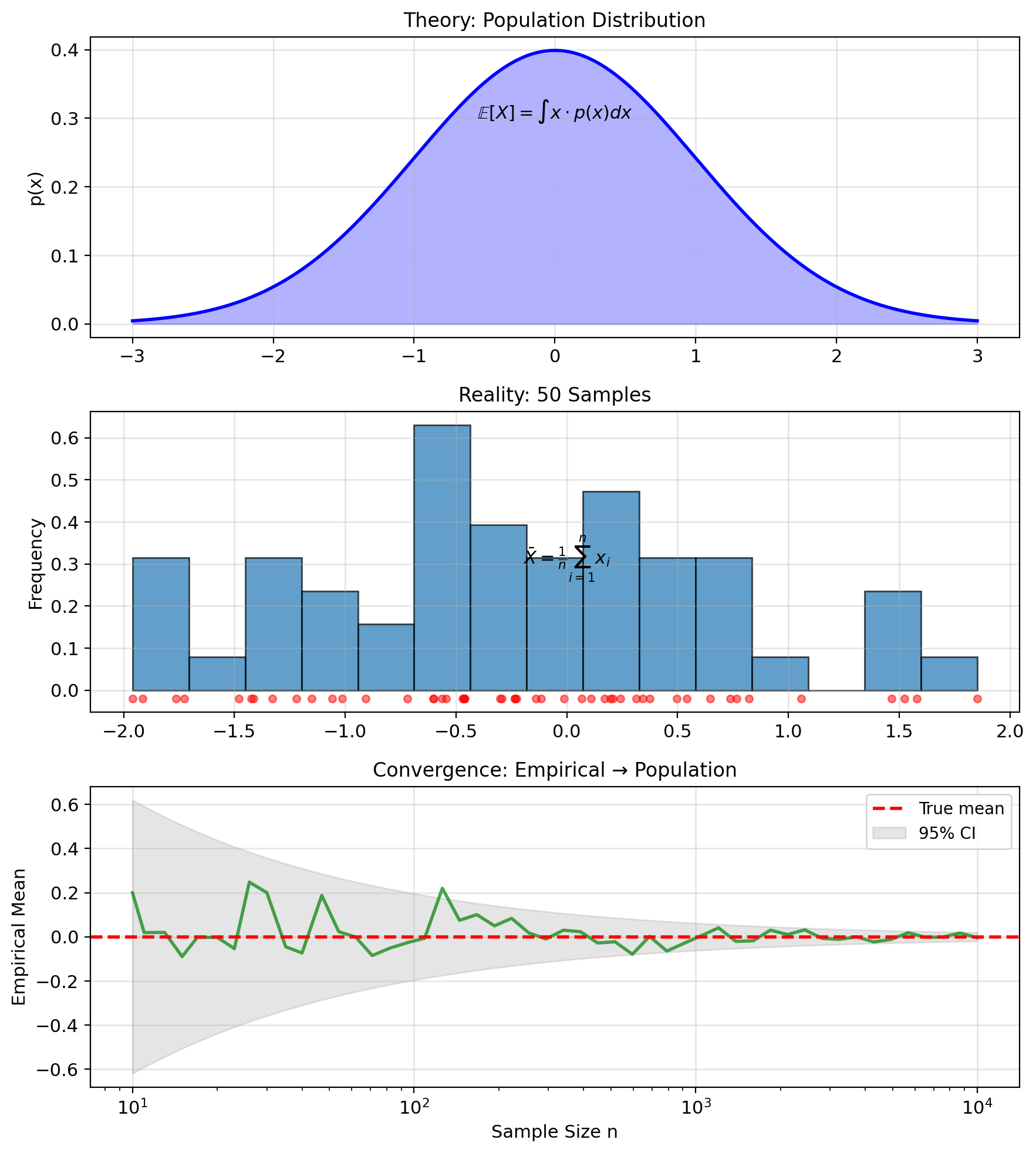
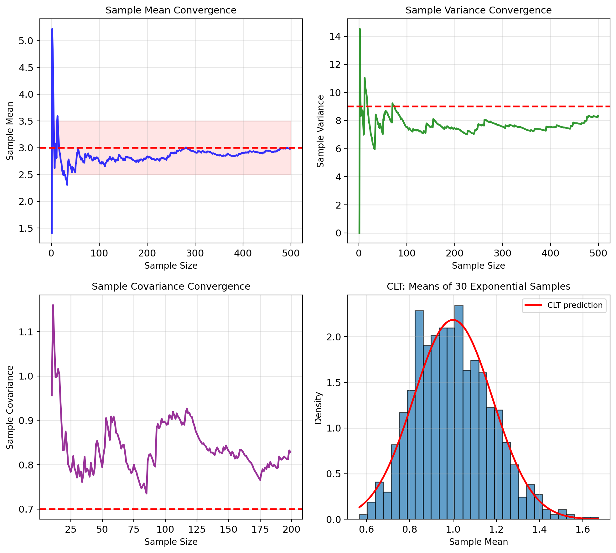
Sample Averages Converge to Population Averages
Population moments – require \(p(x)\): \[\mathbb{E}[X] = \int x \cdot p(x) \, dx\] \[\text{Var}(X) = \int (x - \mathbb{E}[X])^2 p(x) \, dx\]
Sample moments – require only data: \[\bar{X} = \frac{1}{n} \sum_{i=1}^n x_i\] \[S_X^2 = \frac{1}{n} \sum_{i=1}^n (x_i - \bar{X})^2\]
Law of Large Numbers: \[\bar{X} \xrightarrow{a.s.} \mathbb{E}[X]\]
Central Limit Theorem: \[\sqrt{n}(\bar{X} - \mathbb{E}[X]) \xrightarrow{d} \mathcal{N}(0, \sigma^2)\]
Monte Carlo approximation: Integrals become sums over samples
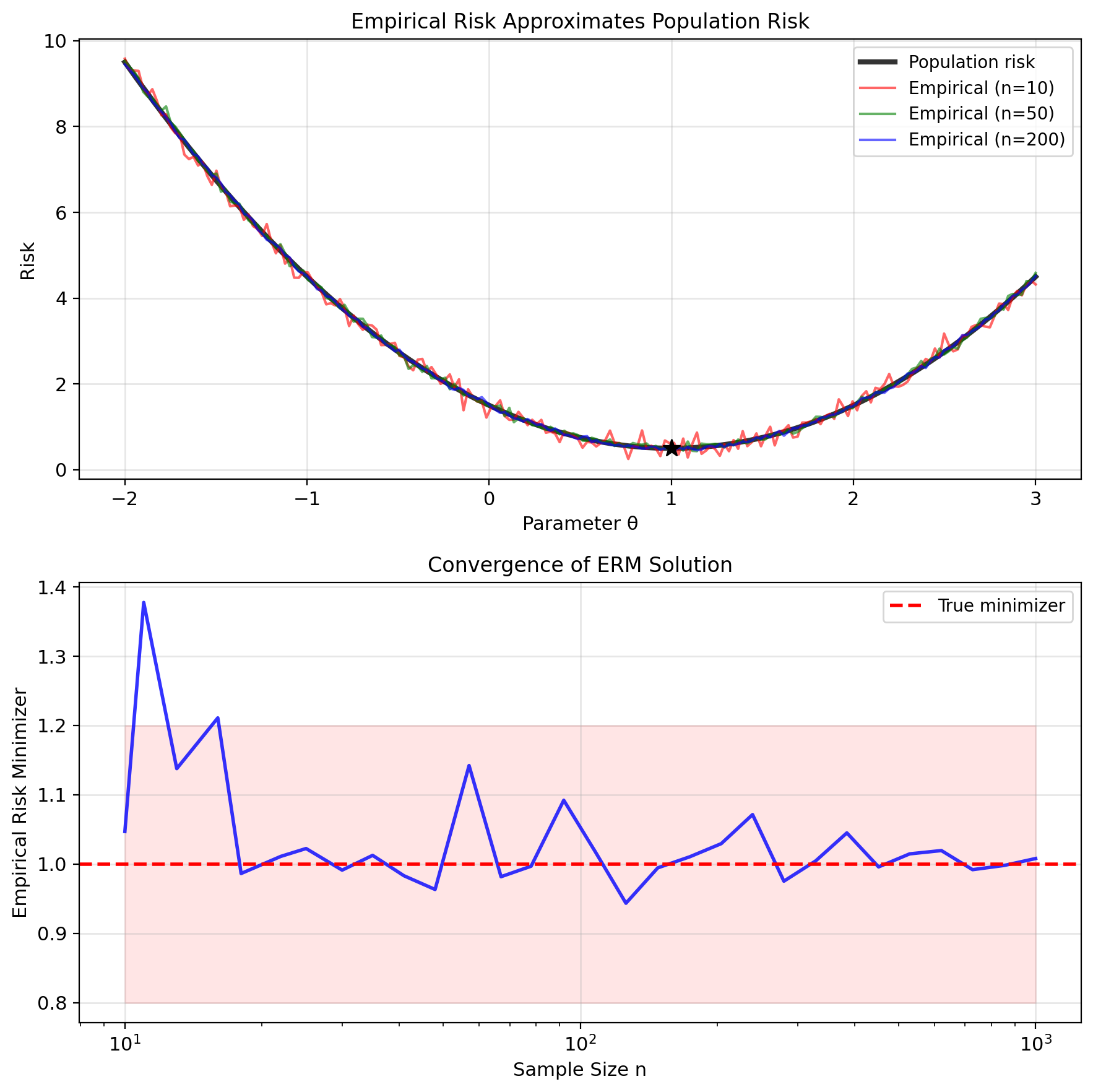
Empirical Risk Minimization
Population risk (what we want to minimize): \[R(f) = \mathbb{E}_{(X,Y)}[\ell(Y, f(X))]\] \[= \int\int \ell(y, f(x)) \, p(x,y) \, dx \, dy\]
Cannot compute without knowing \(p(x,y)\)
Empirical risk (what we can compute): \[\hat{R}_n(f) = \frac{1}{n} \sum_{i=1}^n \ell(y_i, f(x_i))\]
(Empirical Risk Minimization) ERM: \[\hat{f}_n = \arg\min_{f \in \mathcal{F}} \hat{R}_n(f)\]
Convergence guarantee: Under regularity conditions, \[R(\hat{f}_n) - \inf_{f \in \mathcal{F}} R(f) \xrightarrow{P} 0\]
Sample minimizer converges to population minimizer as \(n \to \infty\)
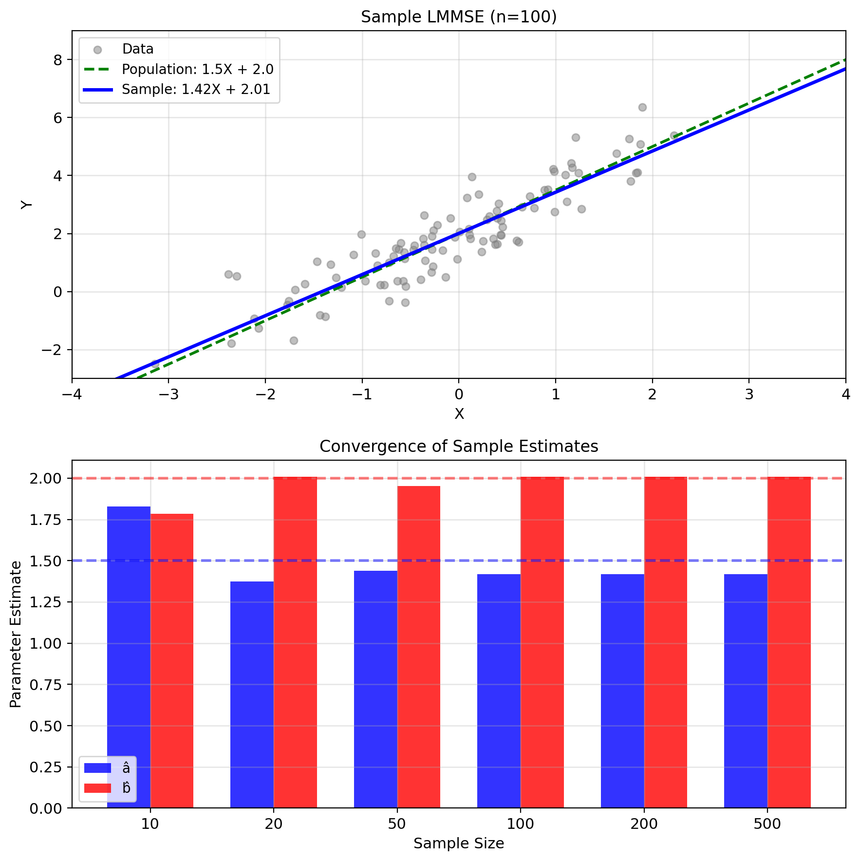
LMMSE with Sample Moments
Population LMMSE: \[a^* = \frac{\text{Cov}(X,Y)}{\text{Var}(X)}, \quad b^* = \mathbb{E}[Y] - a^*\mathbb{E}[X]\]
Sample LMMSE: \[\hat{a} = \frac{\hat{K}_{XY}}{\hat{K}_X}, \quad \hat{b} = \bar{Y} - \hat{a}\bar{X}\]
where:
- \(\bar{X} = \frac{1}{n}\sum x_i\), \(\bar{Y} = \frac{1}{n}\sum y_i\)
- \(\hat{K}_X = \frac{1}{n}\sum (x_i - \bar{X})^2\)
- \(\hat{K}_{XY} = \frac{1}{n}\sum (x_i - \bar{X})(y_i - \bar{Y})\)
This is linear regression.
Same formula, different source:
- Theory: Population moments
- Practice: Sample moments
Consistency: \(\hat{a} \xrightarrow{P} a^*\), \(\hat{b} \xrightarrow{P} b^*\) as \(n \to \infty\)
Why Squared Loss?
The framework so far: Minimize a loss over data \[\hat{f} = \arg\min_{f} \frac{1}{n}\sum_{i=1}^n \ell(y_i, f(x_i))\]
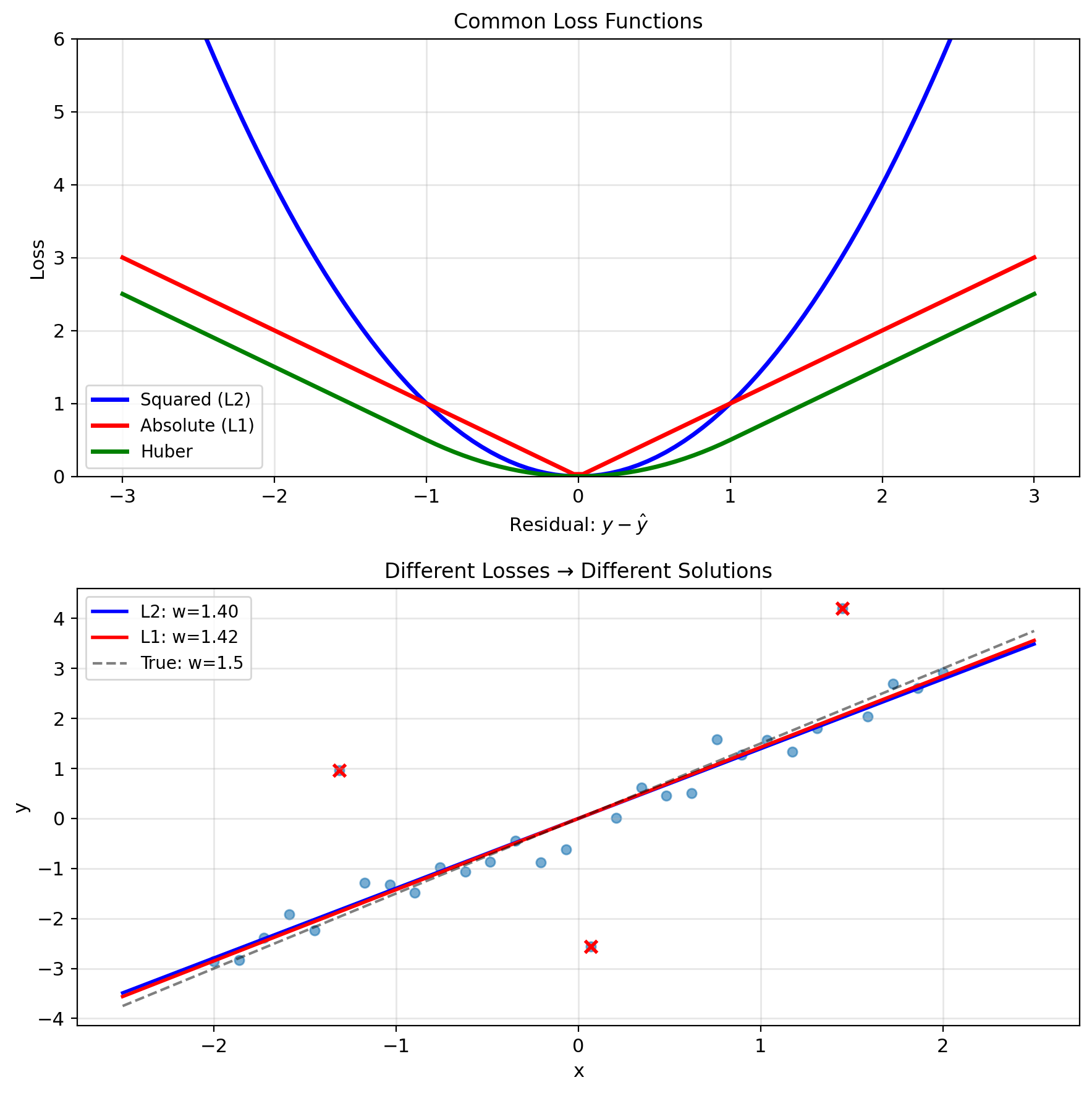
But which loss? Different choices give different estimators:
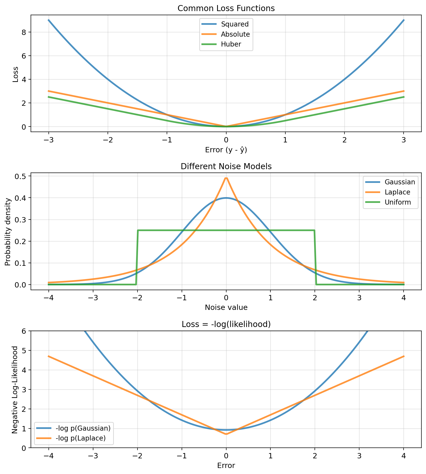
- Squared: \((y - \hat{y})^2\)
- Absolute: \(|y - \hat{y}|\)
- Huber: Combination of both
The choice encodes assumptions about how noise enters the data
Maximum likelihood makes this explicit:
- Specify a probabilistic model for data generation
- The loss function emerges from the model
- Different noise → different losses
Modeling Data Generation
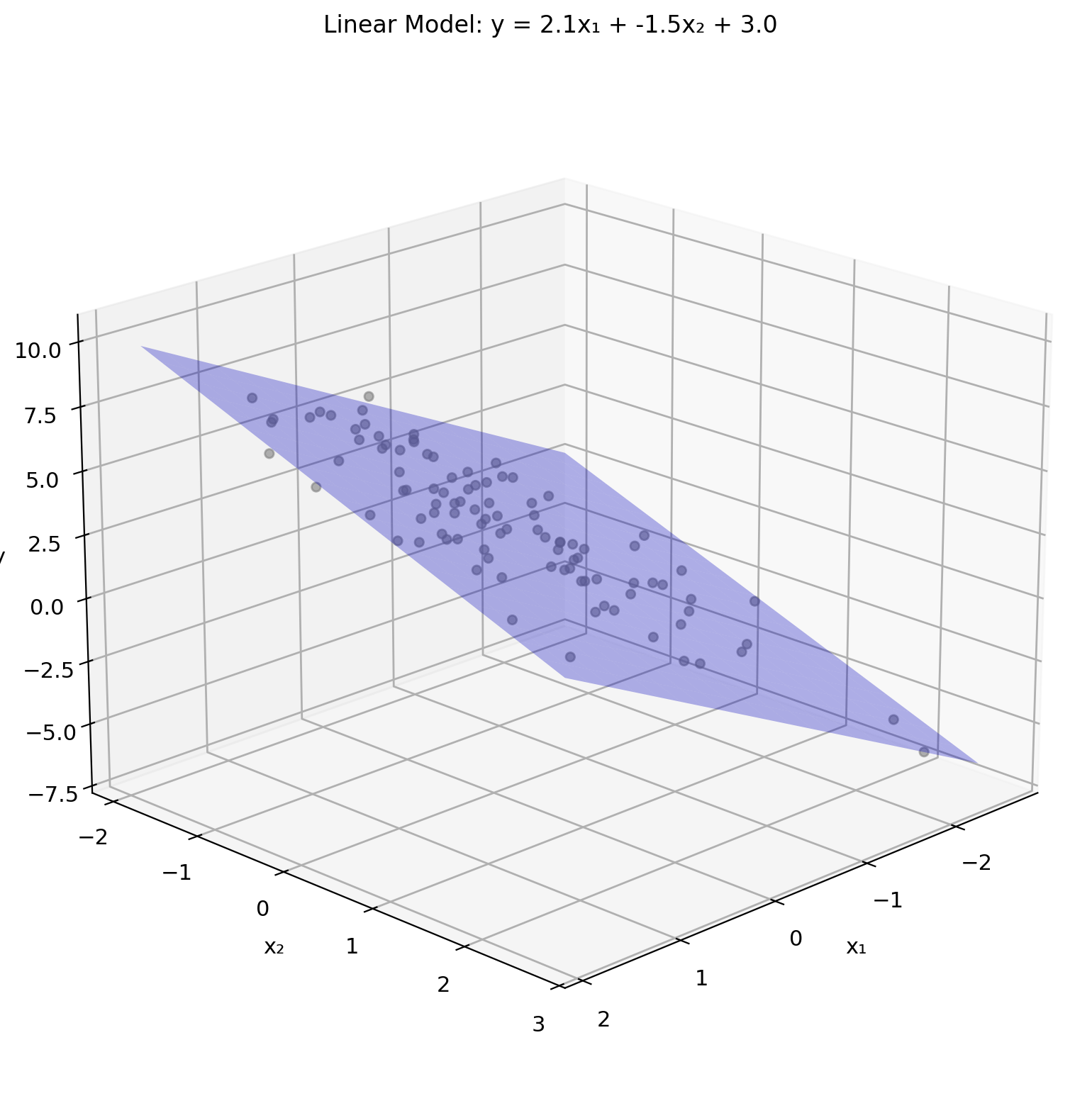
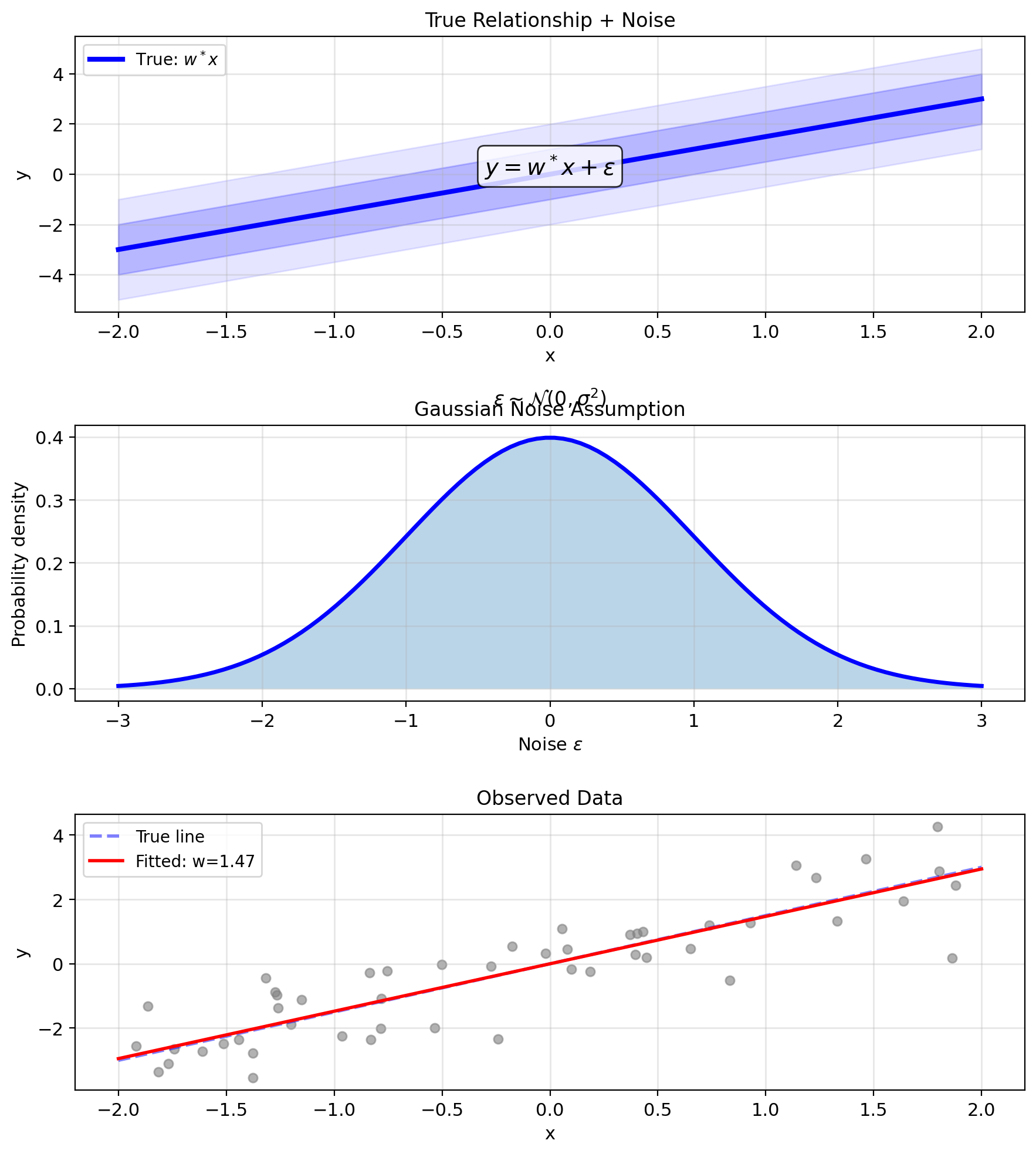
Assume data comes from a process: \[y = w^T x + \epsilon\]
where \(\epsilon\) is random noise
What we observe:
- True relationship: \(w^T x\)
- Plus noise: \(\epsilon\)
Key questions:
- What distribution for \(\epsilon\)?
- How does this affect estimation?
Common assumption: \(\epsilon \sim \mathcal{N}(0, \sigma^2)\)
Why Gaussian?
- Central limit theorem: sum of many small effects
- Maximum entropy for fixed variance
- Mathematical tractability
- Often reasonable in practice
Probabilistic View of Regression
Model: \(y = w^T x + \epsilon\), where \(\epsilon \sim \mathcal{N}(0, \sigma^2)\)
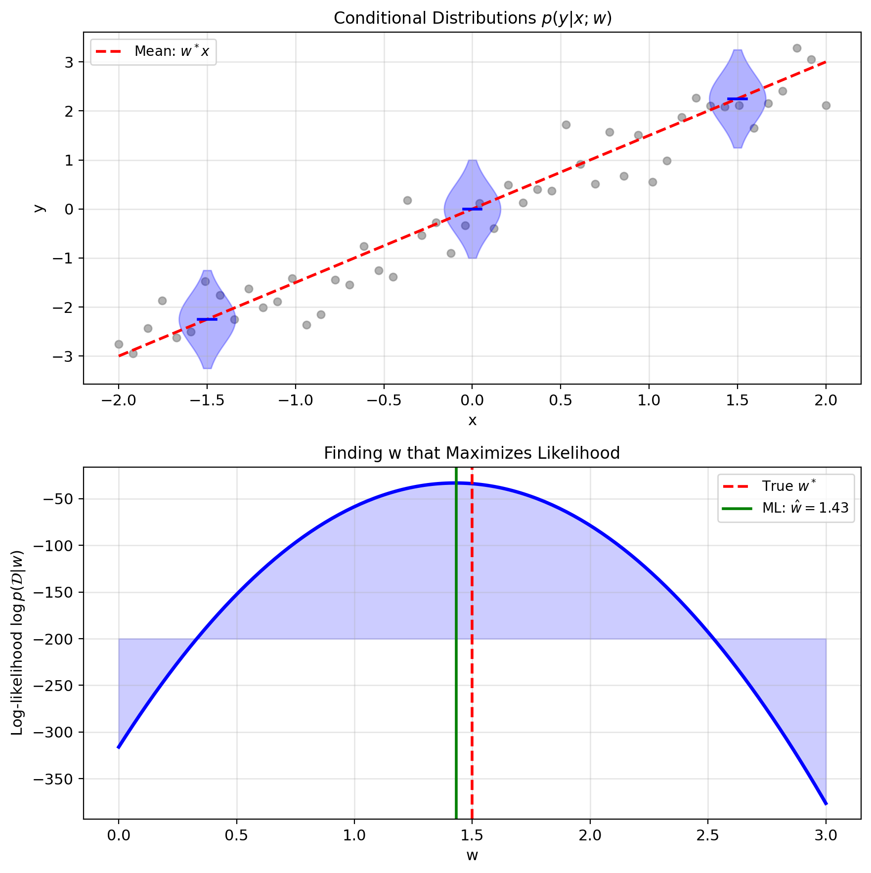
This implies \(y|x\) is Gaussian: \[y|x \sim \mathcal{N}(w^T x, \sigma^2)\]
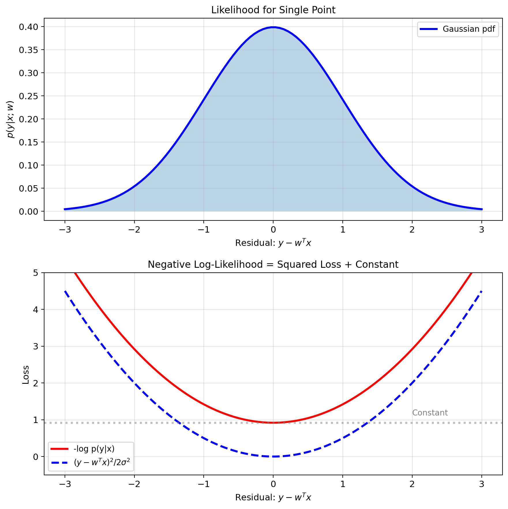
Probability of observing \(y\) given \(x\): \[p(y|x; w) = \frac{1}{\sqrt{2\pi\sigma^2}} \exp\left(-\frac{(y - w^T x)^2}{2\sigma^2}\right)\]
For entire dataset \(\mathcal{D} = \{(x_i, y_i)\}_{i=1}^n\):
Assuming independent samples: \[p(\mathcal{D}|w) = \prod_{i=1}^n p(y_i|x_i; w)\]
Maximum likelihood principle: Find \(w\) that makes observed data most probable: \[\hat{w}_{\text{ML}} = \arg\max_w p(\mathcal{D}|w)\]
From Likelihood to Least Squares
Log-likelihood: \[\ell(w) = \log p(\mathcal{D}|w) = \sum_{i=1}^n \log p(y_i|x_i; w)\]
Substitute Gaussian pdf: \[\ell(w) = \sum_{i=1}^n \log \left(\frac{1}{\sqrt{2\pi\sigma^2}} e^{-\frac{(y_i - w^T x_i)^2}{2\sigma^2}}\right)\]
Simplify: \[\ell(w) = -\frac{n}{2}\log(2\pi\sigma^2) - \frac{1}{2\sigma^2}\sum_{i=1}^n(y_i - w^T x_i)^2\]
To maximize \(\ell(w)\):
- First term: constant w.r.t. \(w\)
- Second term: minimize \(\sum_i(y_i - w^T x_i)^2\)
Result: MLE = Least squares
\[\hat{w}_{\text{ML}} = \arg\min_w \sum_{i=1}^n(y_i - w^T x_i)^2\]
Gaussian noise assumption leads to squared loss
MLE Gives Normal Equations
Maximize log-likelihood: \[\hat{w} = \arg\max_w \ell(w) = \arg\min_w ||y - Xw||^2\]
Take gradient of loss: \[\nabla_w \left[\frac{1}{2}||y - Xw||^2\right] = -X^T(y - Xw)\]
Set to zero (critical point): \[-X^T(y - Xw) = 0\] \[X^T Xw = X^T y\]
Normal equations (same result as before): \[\boxed{\hat{w}_{\text{ML}} = (X^T X)^{-1} X^T y}\]
So:
- Least squares has probabilistic justification
- Assumes Gaussian noise
- Different noise → different estimator
- MLE provides principled framework
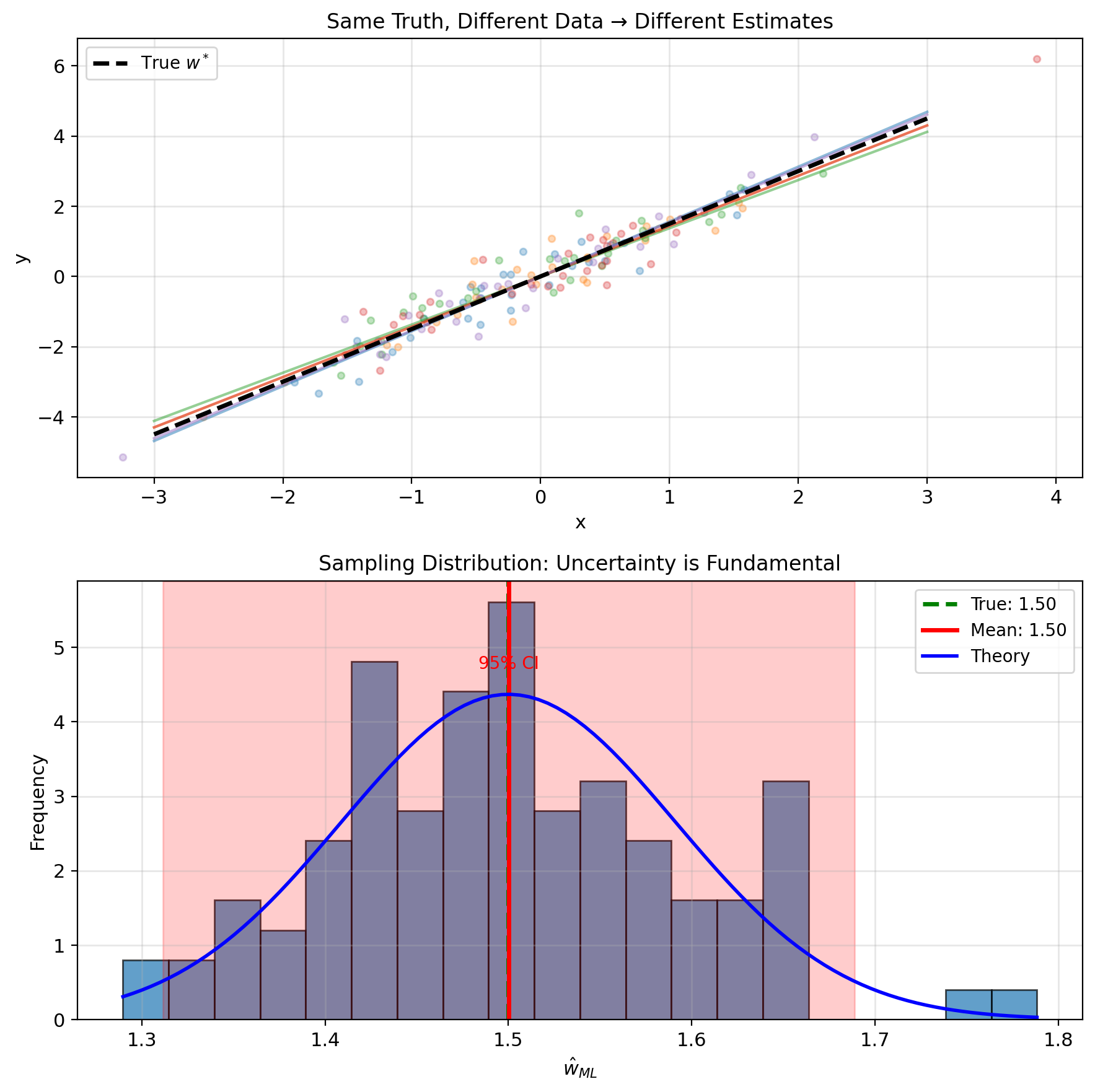
Beyond Point Estimates: Uncertainty Matters
MLE gives us \(\hat{w}\), but:
- How confident are we?
- Could true \(w^*\) be far from \(\hat{w}\)?
- Which parameters are well-determined?
Sources of uncertainty:
- Finite sample size
- Noise level \(\sigma^2\)
- Data distribution (design matrix \(X\))
Statistical inference framework:
- Point estimate: \(\hat{w}_{\text{ML}}\) (where)
- Uncertainty: \(\text{Cov}(\hat{w})\) (how sure)
- Confidence regions: Where \(w^*\) likely lies
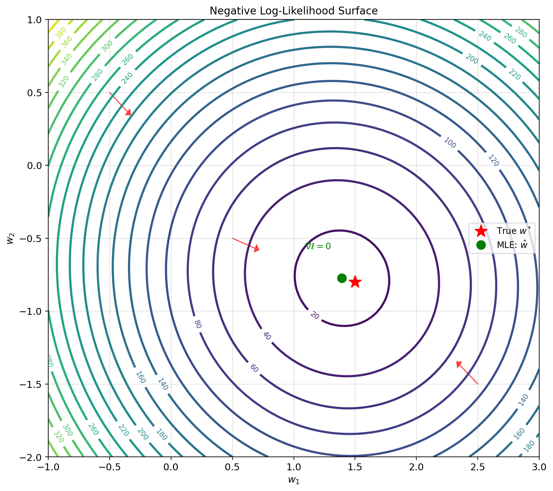
MLE is a random variable \[\hat{w} = (X^TX)^{-1}X^Ty = (X^TX)^{-1}X^T(Xw^* + \epsilon)\] \[= w^* + (X^TX)^{-1}X^T\epsilon\]
Distribution of \(\hat{w}\) depends on distribution of \(\epsilon\)
Fisher Information: Quantifies how much information data contains about parameters
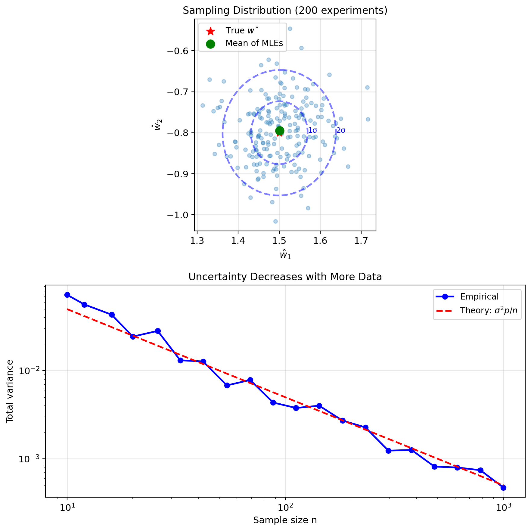
Fisher Information and Uncertainty
Fisher information matrix: \[\mathbf{I}(w) = -\mathbb{E}\left[\frac{\partial^2 \ell(w)}{\partial w \partial w^T}\right]\]
For linear regression: \[\mathbf{I}(w) = \frac{1}{\sigma^2}X^T X\]
Measures “information” about \(w\) in data
Covariance of ML estimator: \[\text{Cov}(\hat{w}_{\text{ML}}) = \mathbf{I}^{-1} = \sigma^2(X^T X)^{-1}\]
- Large \(X^T X\) → small variance (precise)
- Small \(X^T X\) → large variance (uncertain)
- Ill-conditioned \(X^T X\) → very uncertain
Confidence regions: \[(\hat{w} - w^*)^T \mathbf{I} (\hat{w} - w^*) \sim \chi^2_p\]
Forms ellipsoid around estimate
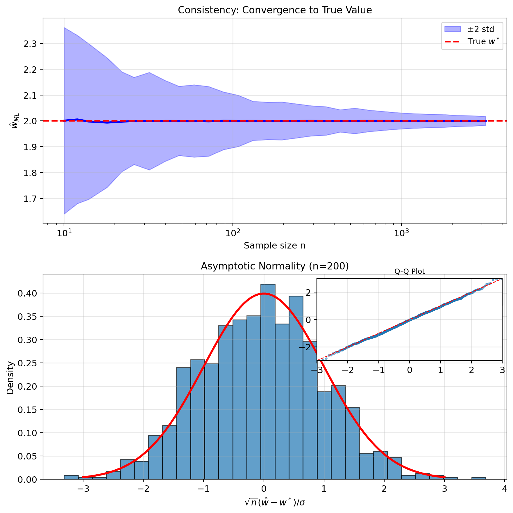
Properties of ML Estimators
Consistency: \[\hat{w}_n \xrightarrow{p} w^* \text{ as } n \to \infty\]
MLE converges to true value with enough data
Asymptotic normality: \[\sqrt{n}(\hat{w}_n - w^*) \xrightarrow{d} \mathcal{N}(0, \sigma^2 K^{-1})\]
where \(K = \lim_{n \to \infty} \frac{1}{n}X^T X\)
Efficiency:
- Achieves minimum possible variance
- Cramér-Rao bound: \(\text{Var}(\hat{w}) \geq \mathbf{I}^{-1}\)
- MLE achieves this bound (asymptotically)
Invariance: If \(\hat{w}\) is MLE of \(w\), then:
- \(g(\hat{w})\) is MLE of \(g(w)\)
- Example: \(||\hat{w}||^2\) is MLE of \(||w||^2\)
Linear Model for Regression
Notation: Weight vector \(w\), bias \(b\) (replacing scalar LMMSE parameters \(a, b\))
Model structure: \[\hat{y} = w^T x + b\]
where:
- \(x \in \mathbb{R}^p\): feature vector
- \(w \in \mathbb{R}^p\): weight vector
- \(b \in \mathbb{R}\): bias/intercept
- \(\hat{y} \in \mathbb{R}\): prediction
Vectorized over dataset: \[\hat{\mathbf{y}} = \mathbf{X}w + b\mathbf{1}\]
- \(\mathbf{X} \in \mathbb{R}^{n \times p}\): data matrix
- \(\mathbf{y} \in \mathbb{R}^n\): target vector
- \(\mathbf{1} \in \mathbb{R}^n\): vector of ones
Augmented notation (“absorb” bias): \[\tilde{x} = \begin{bmatrix} 1 \\ x \end{bmatrix}, \quad \tilde{w} = \begin{bmatrix} b \\ w \end{bmatrix}\]
Then: \(\hat{y} = \tilde{w}^T \tilde{x}\)
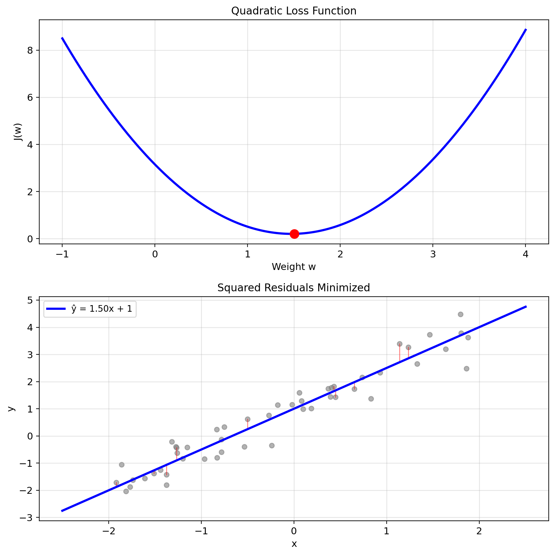
Squared Loss on Finite Data
Empirical risk (squared loss): \[J(w) = \frac{1}{n} \sum_{i=1}^n (y_i - \underbrace{w^T x_i + b}_{\hat{y}_i})^2\]
Matrix form: \[J(w) = \frac{1}{n} ||y - Xw||^2\]
Expanded: \[J(w) = \frac{1}{n}(y - Xw)^T(y - Xw)\] \[= \frac{1}{n}(y^Ty - 2y^TXw + w^TX^TXw)\]
This is a quadratic in \(w\): \[J(w) = \frac{1}{n}(w^T\mathbf{A}w - 2\mathbf{b}^Tw + c)\]
where:
- \(\mathbf{A} = X^TX\) (always positive semidefinite)
- \(\mathbf{b} = X^Ty\)
- \(c = y^Ty\)
Convexity: \(\nabla^2 J = \frac{2}{n}X^TX \succeq 0\)
Setting Up the Normal Equations
Minimize: \(J(w) = \frac{1}{n}||y - Xw||^2\)
Take gradient: \[\nabla_w J = \frac{2}{n}X^T(Xw - y)\]
Set to zero: \[X^T(Xw - y) = 0\]
Normal equations: \[\boxed{X^TXw = X^Ty}\]
Key observations:
- \(X^TX \in \mathbb{R}^{p \times p}\): Gram matrix
- \(X^Ty \in \mathbb{R}^p\): cross-correlation
- System is \(p\) equations in \(p\) unknowns
- Unique solution if \(X^TX\) invertible
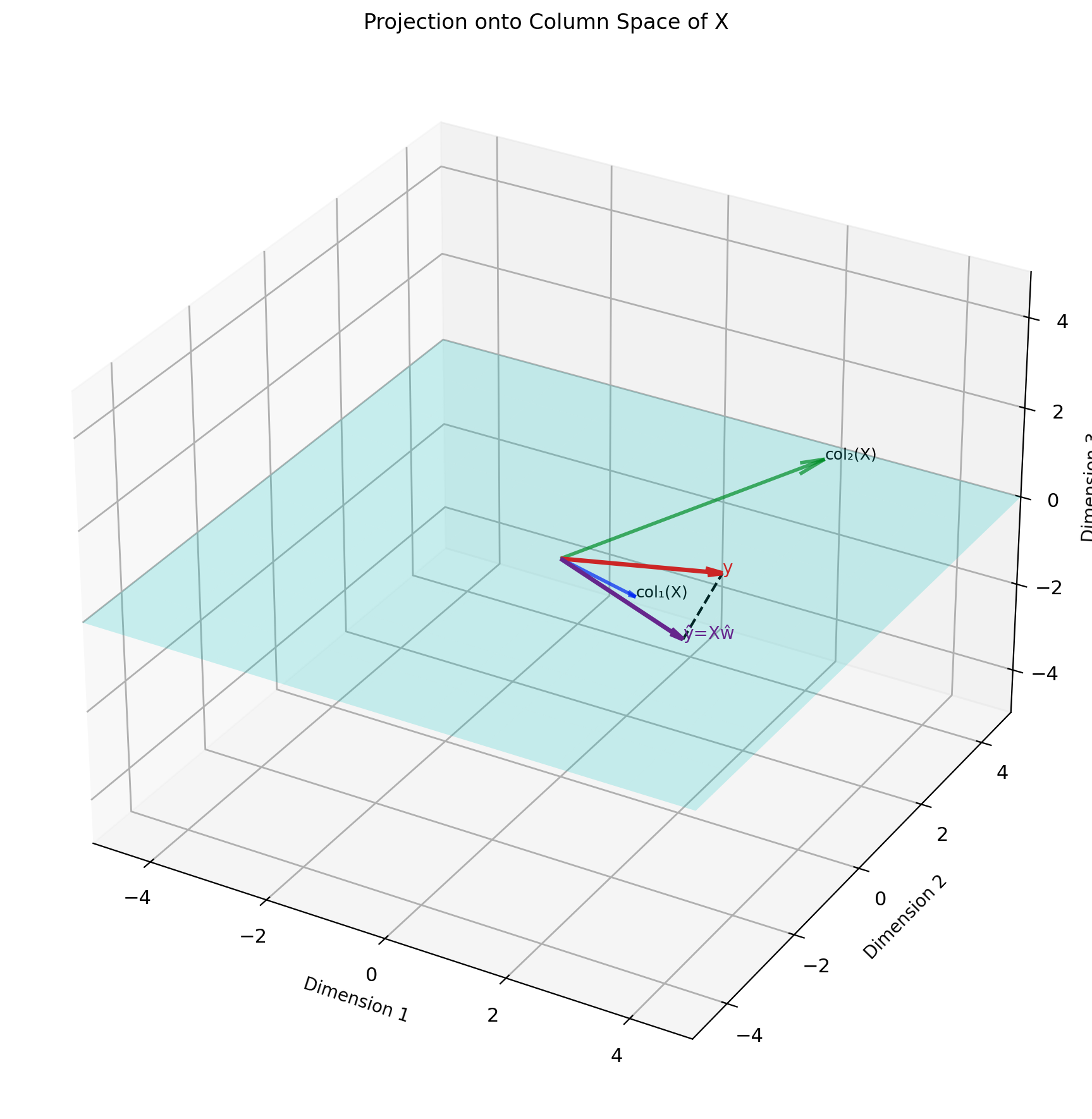
Hence name: Error orthogonal (normal) to column space of \(X\)
Solving the Normal Equations
Solution (when \(X^TX\) invertible): \[w = (X^TX)^{-1}X^Ty\]
Moore-Penrose pseudoinverse: \[X^+ = (X^TX)^{-1}X^T\]
So: \(w = X^+y\)
Properties of \(X^+\):
- \(X^+X = I_p\) (left inverse)
- \(XX^+ = P_X\) (projection onto col(\(X\)))
- Minimizes \(||w||\) if multiple solutions
When is \(X^TX\) invertible?
- Need \(\text{rank}(X) = p\) (full column rank)
- Requires \(n \geq p\) (more data than features)
- Columns of \(X\) linearly independent
Rank deficient case: Use regularization or SVD
Connection to Sample Statistics
Normal equations: \(X^TXw = X^Ty\)
Divide by \(n\): \[\frac{1}{n}X^TXw = \frac{1}{n}X^Ty\]
This gives sample moments:
\[\hat{K}_X w = \hat{k}_{Xy}\]
where:
- \(\hat{K}_X = \frac{1}{n}X^TX\): sample covariance matrix
- \(\hat{k}_{Xy} = \frac{1}{n}X^Ty\): sample cross-covariance
Solution: \[w = \hat{K}_X^{-1} \hat{k}_{Xy}\]
This is empirical LMMSE.
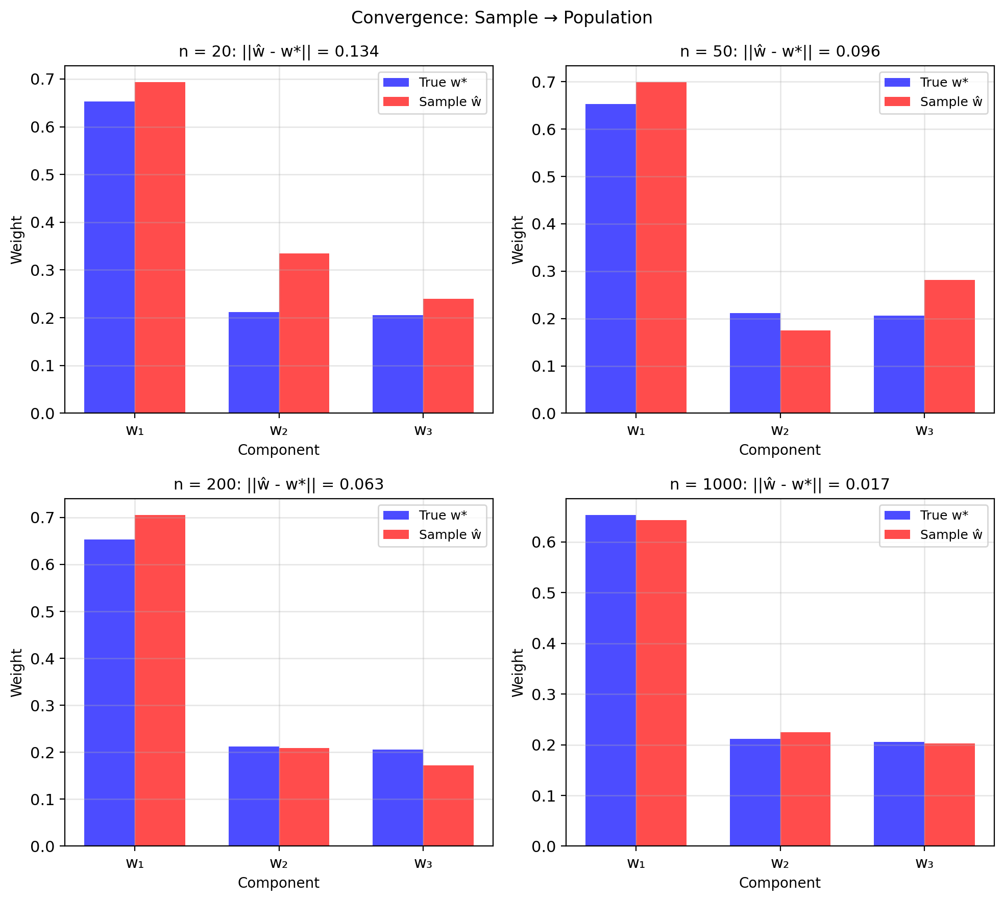
Population: \(w^* = K_X^{-1} k_{Xy}\) Sample: \(\hat{w} = \hat{K}_X^{-1} \hat{k}_{Xy}\)
Consistency: \(\hat{w} \to w^*\) as \(n \to \infty\)
Direct Solution (Computation)
Method 1: Normal equations
w = np.linalg.solve(X.T @ X, X.T @ y)Complexity:
- Form \(X^TX\): \(O(np^2)\)
- Form \(X^Ty\): \(O(np)\)
- Solve system: \(O(p^3)\)
- Total: \(O(np^2 + p^3)\)
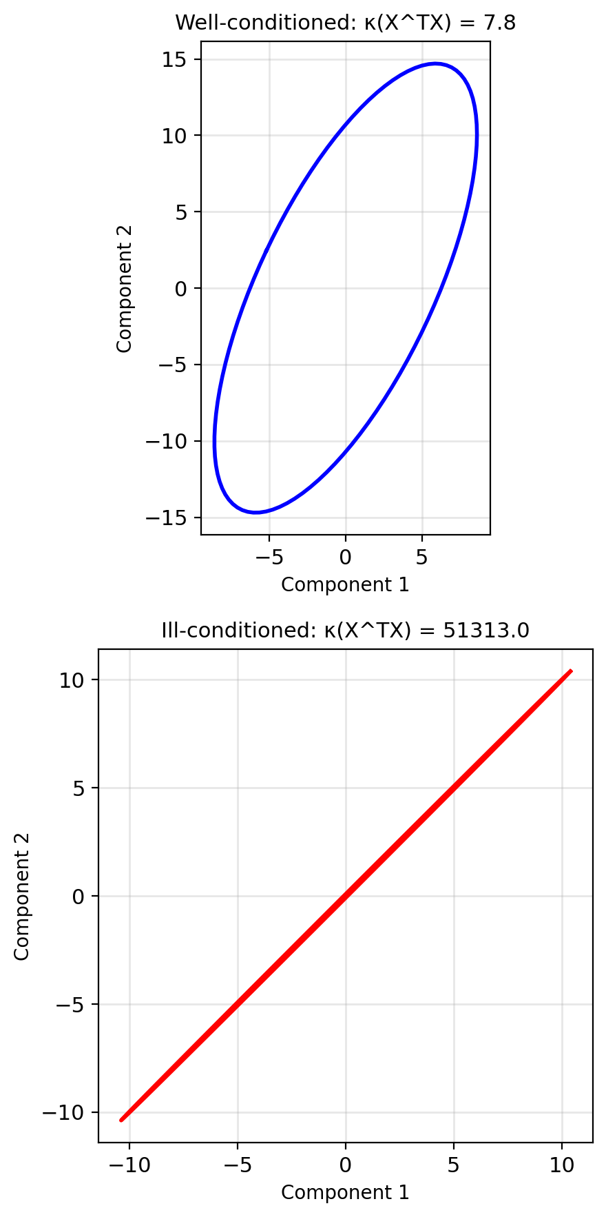
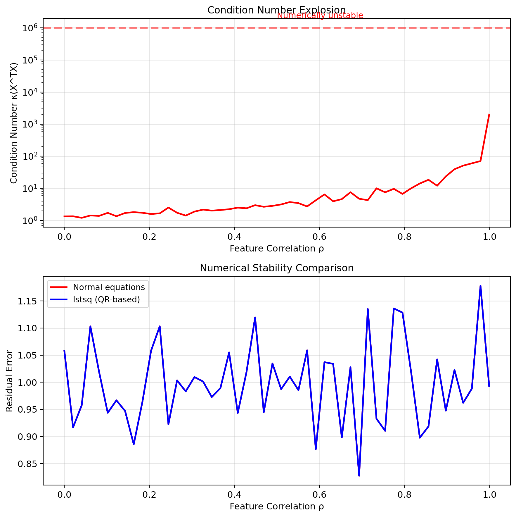
Condition number: \[\kappa(X^TX) = \kappa(X)^2\] Squaring doubles the condition number (in log scale).
QR Decomposition Method
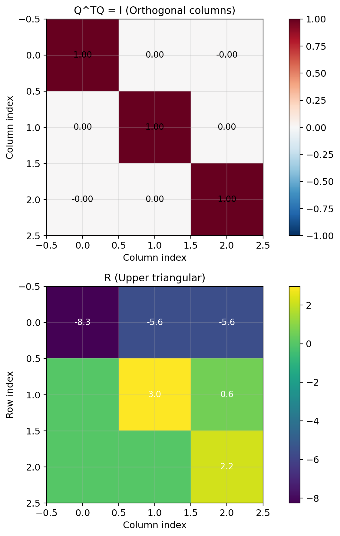
QR factorization: \(X = QR\)
where:
- \(Q \in \mathbb{R}^{n \times p}\): orthogonal columns
- \(R \in \mathbb{R}^{p \times p}\): upper triangular
Solve via QR: \[X^TXw = X^Ty\] \[(QR)^T(QR)w = (QR)^Ty\] \[R^TQ^TQRw = R^TQ^Ty\]
Since \(Q^TQ = I\): \[R^TRw = R^TQ^Ty\]
If \(R\) full rank: \(R^T\) invertible: \[Rw = Q^Ty\]
Back-substitution: Solve triangular system
Complexity: \(O(2np^2)\) but numerically stable
Advantage: Avoids calculating \(X^TX\) explicitly
SVD for Robust Solutions
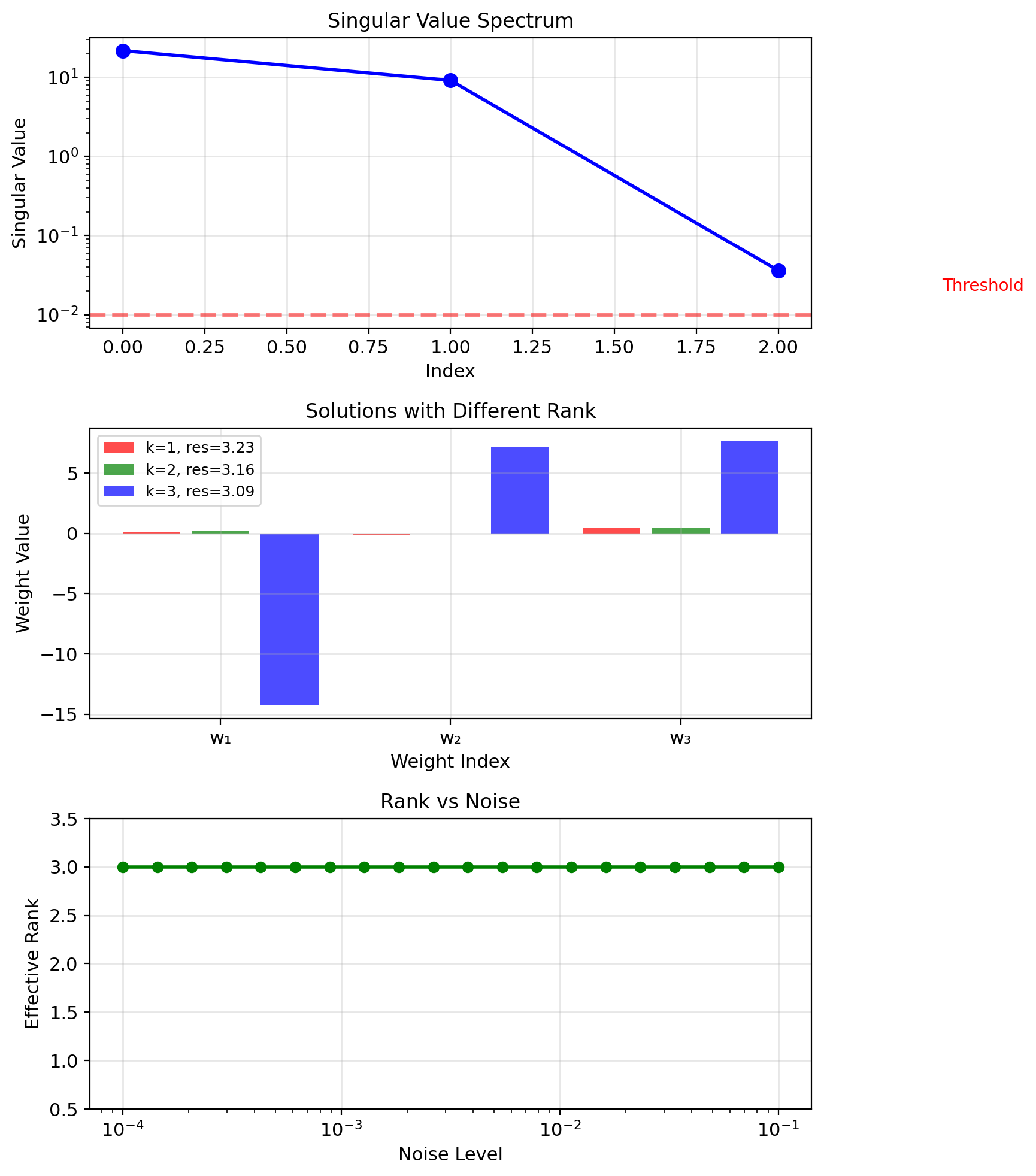
Singular Value Decomposition: \[X = U\Sigma V^T\]
where:
- \(U \in \mathbb{R}^{n \times n}\): left singular vectors
- \(\Sigma \in \mathbb{R}^{n \times p}\): diagonal (singular values)
- \(V \in \mathbb{R}^{p \times p}\): right singular vectors
Solution via SVD: \[w = V\Sigma^+ U^T y\]
where \(\Sigma^+\) = pseudoinverse of \(\Sigma\):
- If \(\sigma_i > \epsilon\): \(\sigma_i^+ = 1/\sigma_i\)
- If \(\sigma_i \leq \epsilon\): \(\sigma_i^+ = 0\)
Truncated SVD (regularization): Keep only \(k\) largest singular values
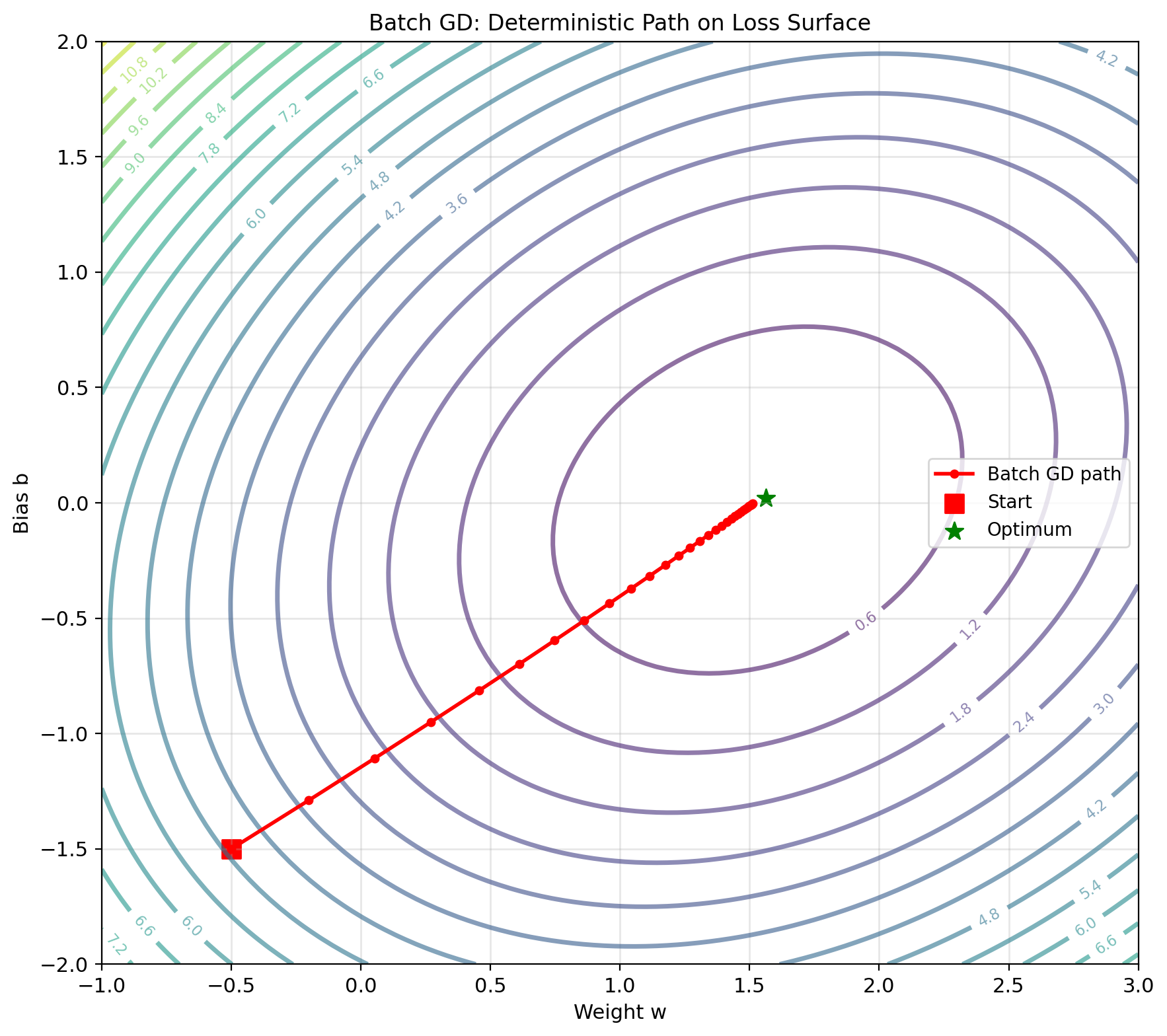
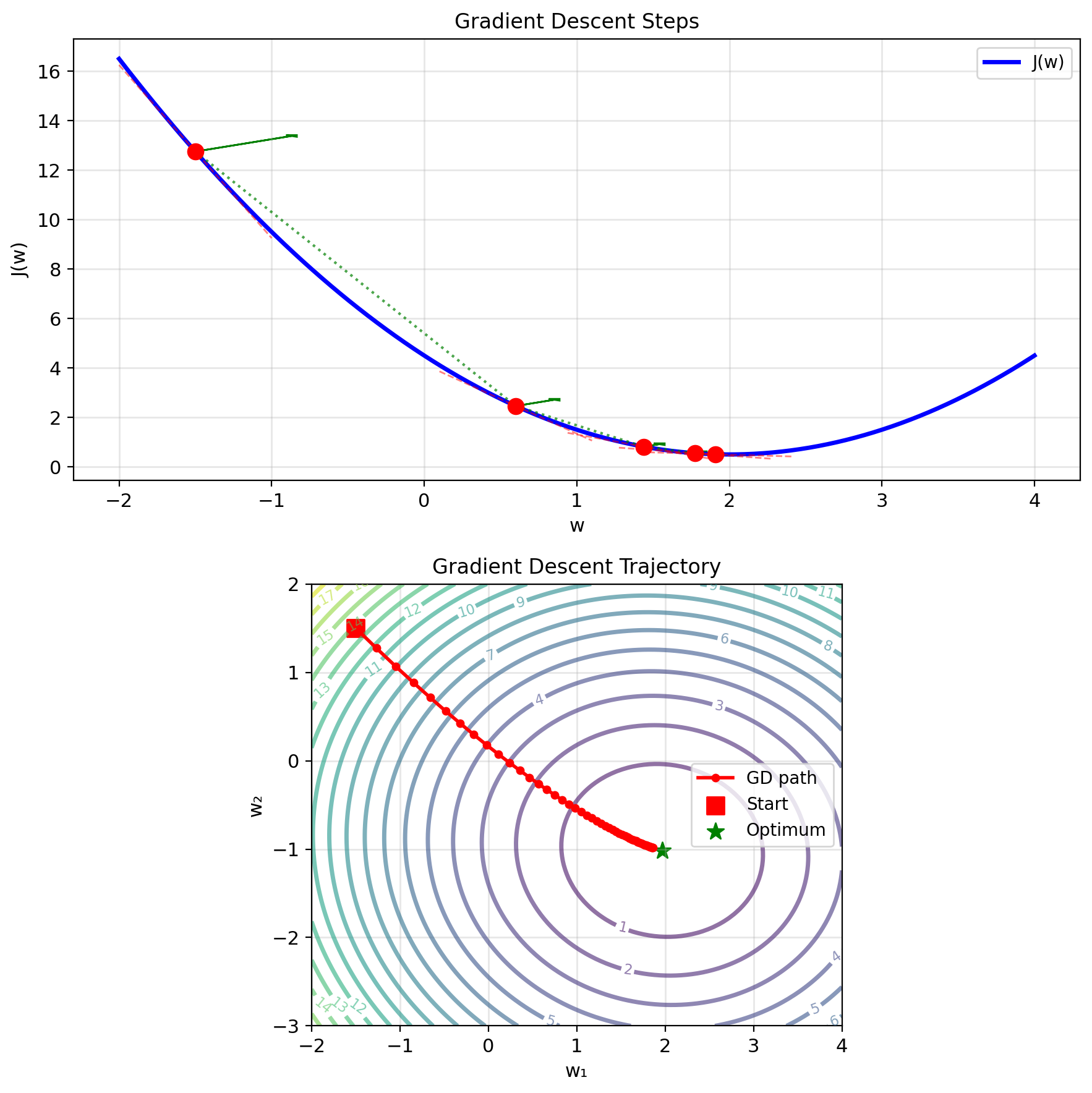
Gradient Descent: Following the Slope
Key idea: Move downhill in direction of steepest descent
Gradient points uphill: \[\nabla J(w) = \frac{2}{n}X^T(Xw - y)\]
Direction of maximum increase of \(J\)
Descent direction: \(-\nabla J(w)\)
Update rule: \[w_{t+1} = w_t - \alpha \nabla J(w_t)\]
where \(\alpha\) = step size / learning rate
Intuition:
- At each point, linearize the function
- Take small step in direction that decreases \(J\) most
- Repeat until convergence
Convergence criterion: \[||\nabla J(w)|| < \epsilon\]
At optimum: \(\nabla J(w^*) = 0\) (critical point)
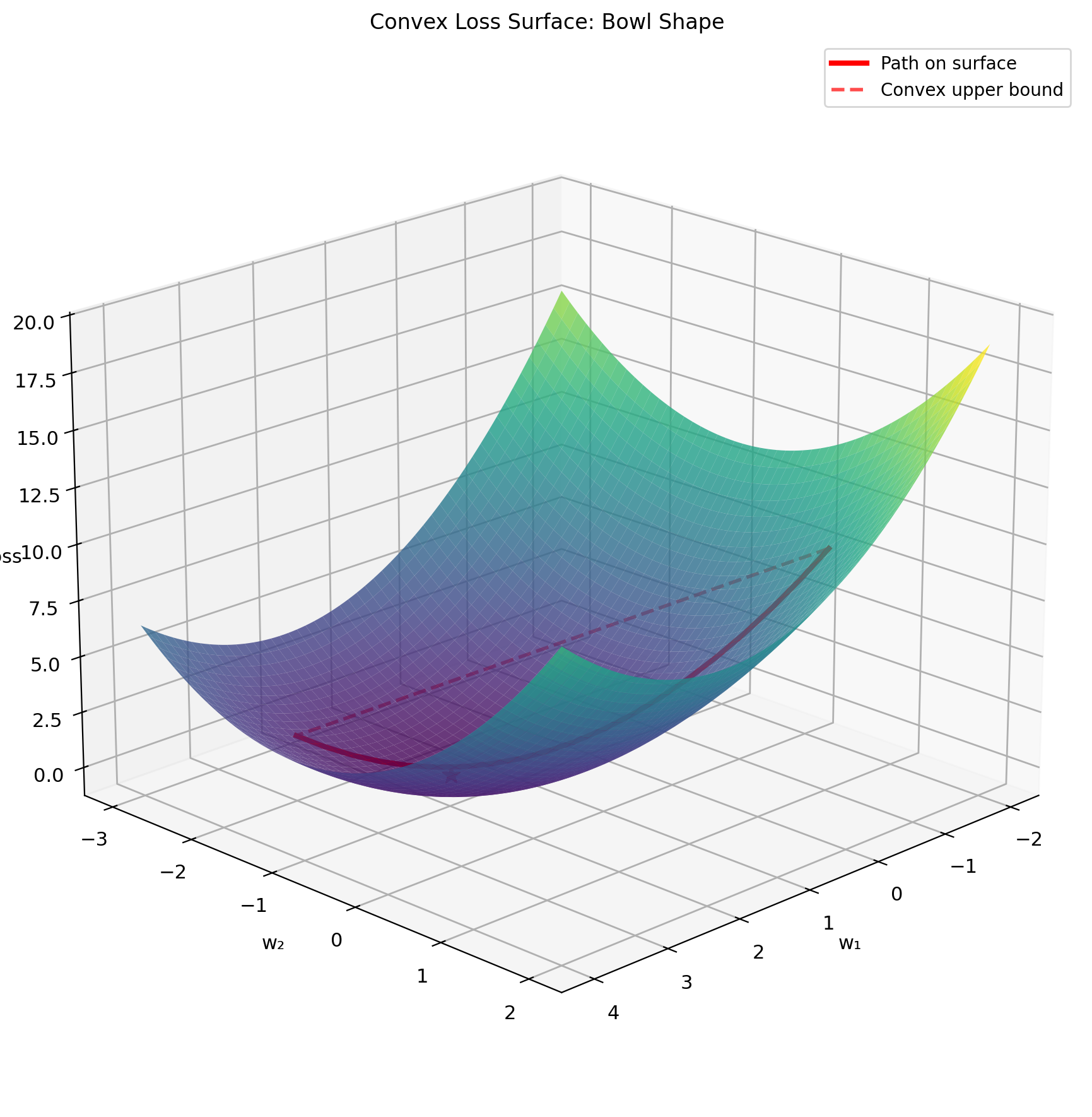
Convexity of Squared Loss
Definition: \(f\) is convex if for all \(\lambda \in [0,1]\): \[f(\lambda w_1 + (1-\lambda)w_2) \leq \lambda f(w_1) + (1-\lambda)f(w_2)\]
Squared loss is convex: \[J(w) = \frac{1}{n}||y - Xw||^2\]
Proof via Hessian: \[\nabla^2 J = \frac{2}{n}X^TX\]
Since \(X^TX \succeq 0\) (positive semidefinite): \[v^T(X^TX)v = ||Xv||^2 \geq 0 \quad \forall v\]
Therefore \(J\) is convex.
- Any local minimum is global minimum
- If minimum exists, it’s unique (if \(X^TX \succ 0\))
- Gradient descent converges to global minimum
- No need for random restarts
Strong convexity if \(X\) full rank: \[J(w) \geq J(w^*) + \frac{\mu}{2}||w - w^*||^2\] where \(\mu = \lambda_{\min}(X^TX)/n > 0\)
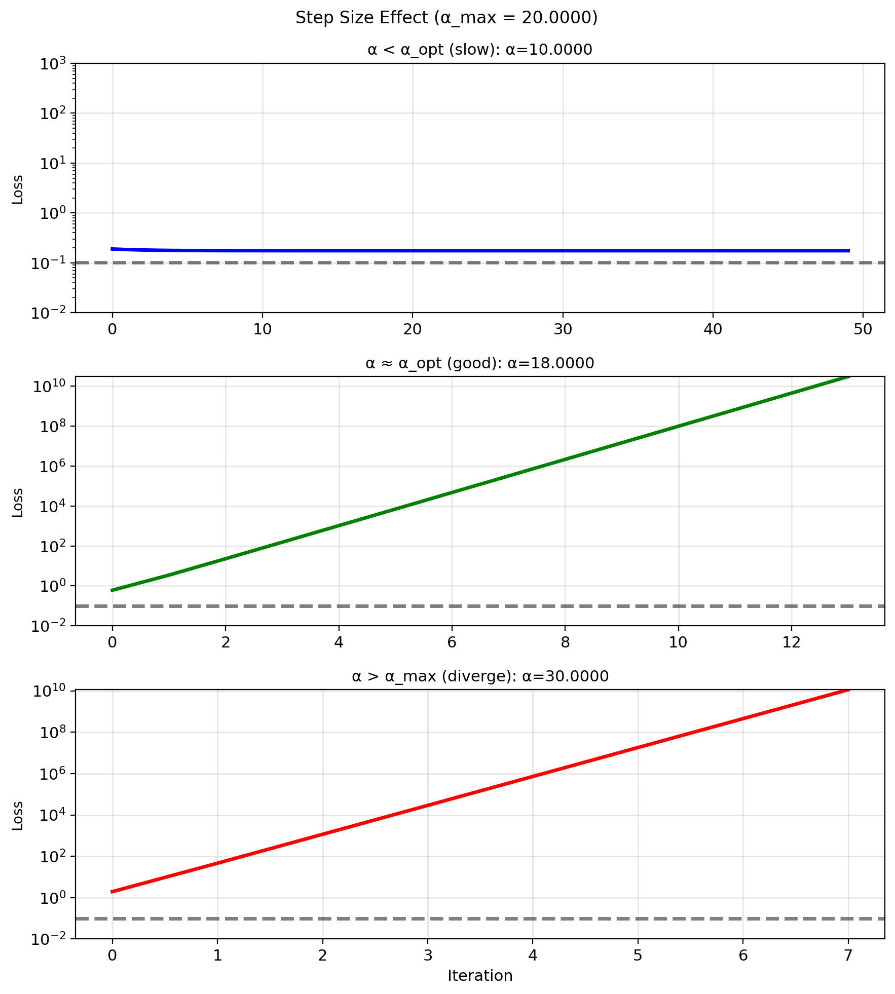
Step Size \(\alpha\) and Convergence
Too small: Slow convergence \[w_{t+1} \approx w_t\]
Too large: Overshoot, divergence \[J(w_{t+1}) > J(w_t)\]
Just right: “Stable” convergence
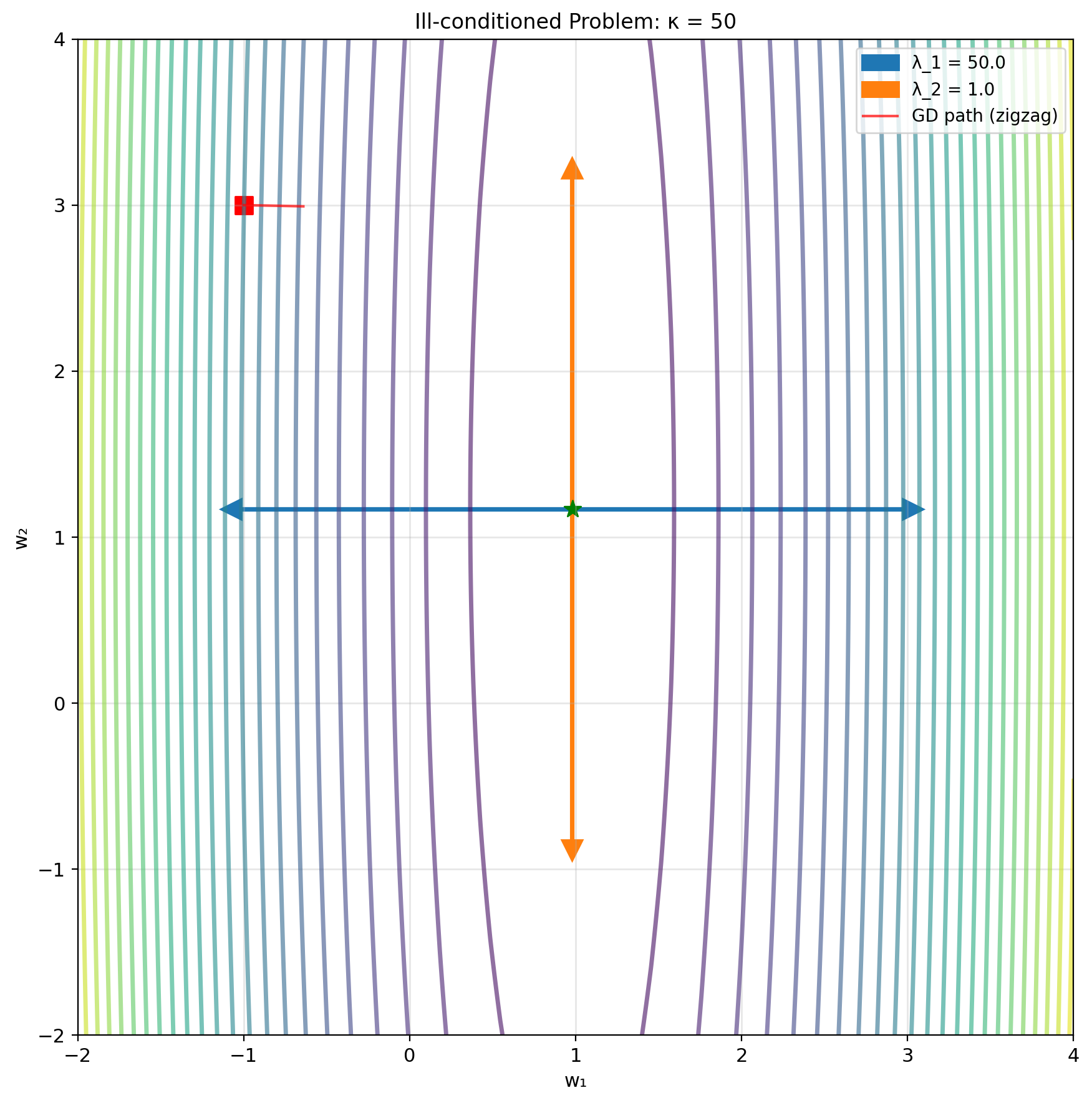
Condition number effect: \[\kappa = \frac{\lambda_{\max}}{\lambda_{\min}}\]
- Small \(\kappa\): Fast convergence
- Large \(\kappa\): Slow, zigzagging
Theoretical bounds: For convergence need: \[0 < \alpha < \frac{2}{\lambda_{\max}(X^TX/n)}\]
“Optimal” step size: \[\alpha^* = \frac{2}{\lambda_{\min} + \lambda_{\max}}\]
Convergence rate: \[||w_t - w^*|| \leq \left(\frac{\kappa - 1}{\kappa + 1}\right)^t ||w_0 - w^*||\]
Eigenvalues and Geometry
Loss surface shape determined by eigenvalues of \(X^TX\)
Principal axes: Eigenvectors of \(X^TX\)
Curvature along axis: Eigenvalue
Gradient descent behavior:
- Fast convergence along high curvature (large \(\lambda\))
- Slow along low curvature (small \(\lambda\))
- Zigzagging when \(\kappa\) large
Preconditioning: Transform to make all eigenvalues equal \[\tilde{X} = XP^{-1}\] where \(P\) chosen so \(\tilde{X}^T\tilde{X} = I\)
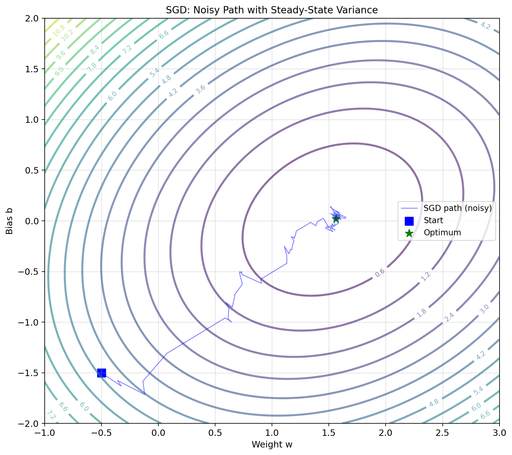
Stochastic Gradient Descent
Use one sample at a time: \[w_{t+1} = w_t - \alpha_t \nabla \ell_{i_t}(w_t)\]
where \(i_t\) randomly selected
For squared loss: \[\nabla \ell_i(w) = -2(y_i - w^T x_i)x_i\]
LMS algorithm (Widrow-Hoff) is SGD for squared loss: \(w_{t+1} = w_t + \mu e_t x_t\)
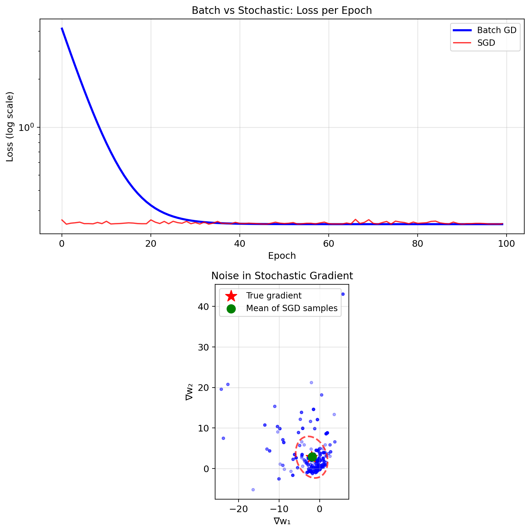
Unbiased gradient estimate: \[\mathbb{E}[\nabla \ell_i(w)] = \nabla J(w)\]
Noise in gradient: \[\text{Var}[\nabla \ell_i] = \mathbb{E}[||\nabla \ell_i||^2] - ||\nabla J||^2\]
Benefits:
- Cheap iteration: \(O(p)\) vs \(O(np)\)
- Online learning capability
- Escape shallow local minima
- Implicit regularization via noise
Batching and SGD Convergence
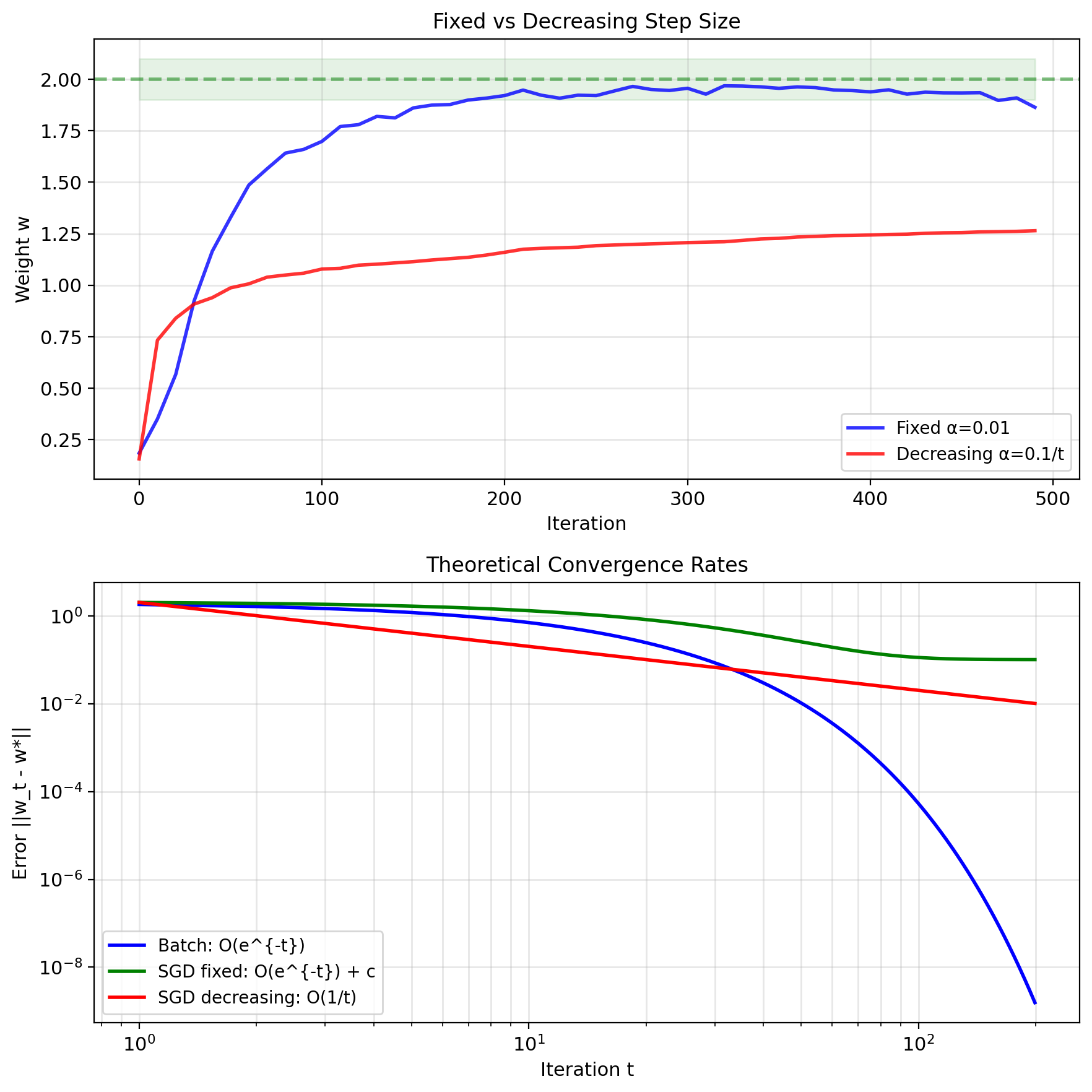
Fixed step size: Converges to neighborhood \[\mathbb{E}[||w_t - w^*||^2] \leq \alpha \sigma^2 + (1-2\alpha\mu)^t||w_0 - w^*||^2\]
where \(\sigma^2\) = gradient noise variance
Decreasing step size: Converges to exact solution
Required conditions (Robbins-Monro): \[\sum_{t=1}^{\infty} \alpha_t = \infty, \quad \sum_{t=1}^{\infty} \alpha_t^2 < \infty\]
Example: \(\alpha_t = \alpha_0/t\)
Convergence rates:
| Method | Rate | Final Error |
|---|---|---|
| Batch GD | \(O(e^{-t})\) | 0 |
| SGD (fixed \(\alpha\)) | \(O(e^{-t})\) | \(O(\alpha)\) |
| SGD (decreasing) | \(O(1/t)\) | 0 |
Variance reduction techniques:
- Mini-batching
- Momentum
- Adaptive methods (Adam, RMSprop)
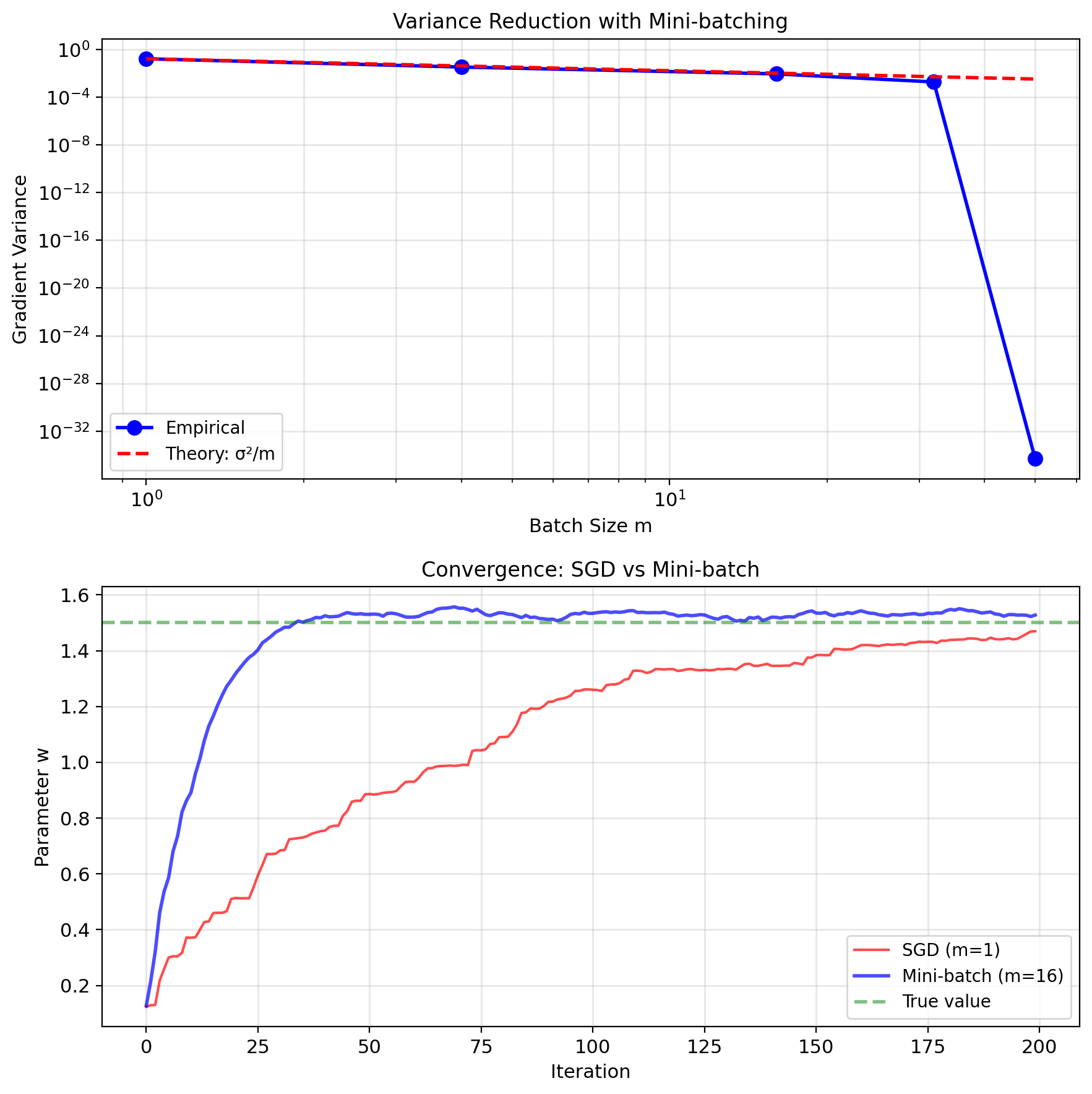
Mini-batching: Variance Reduction
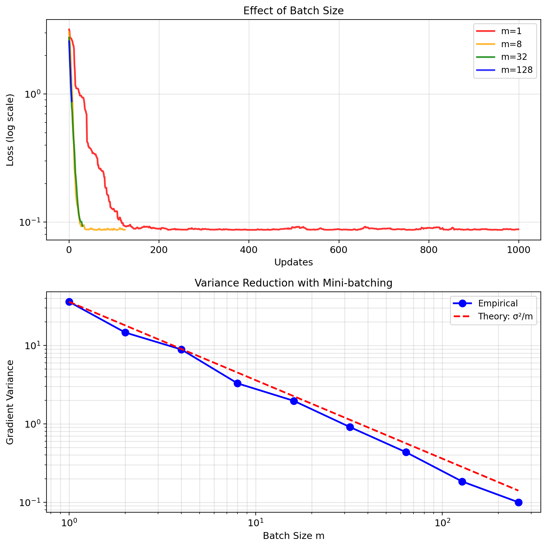
Mini-batch gradient: \[\nabla J_{\mathcal{B}} = \frac{1}{m} \sum_{i \in \mathcal{B}} \nabla \ell_i(w)\]
where \(|\mathcal{B}| = m\) = batch size
Variance reduction: \[\text{Var}[\nabla J_{\mathcal{B}}] = \frac{1}{m}\text{Var}[\nabla \ell_i]\]
Linear speedup in variance reduction.
Benefits:
- Reduces gradient noise by \(\sqrt{m}\)
- Allows larger step sizes
- Better hardware utilization
- Parallelizable
Diminishing returns:
- Computational cost: \(O(m)\)
- Variance reduction: \(O(1/m)\)
Epoch: One pass through dataset
- Batch: 1 update per epoch
- SGD: \(n\) updates per epoch
- Mini-batch: \(n/m\) updates per epoch
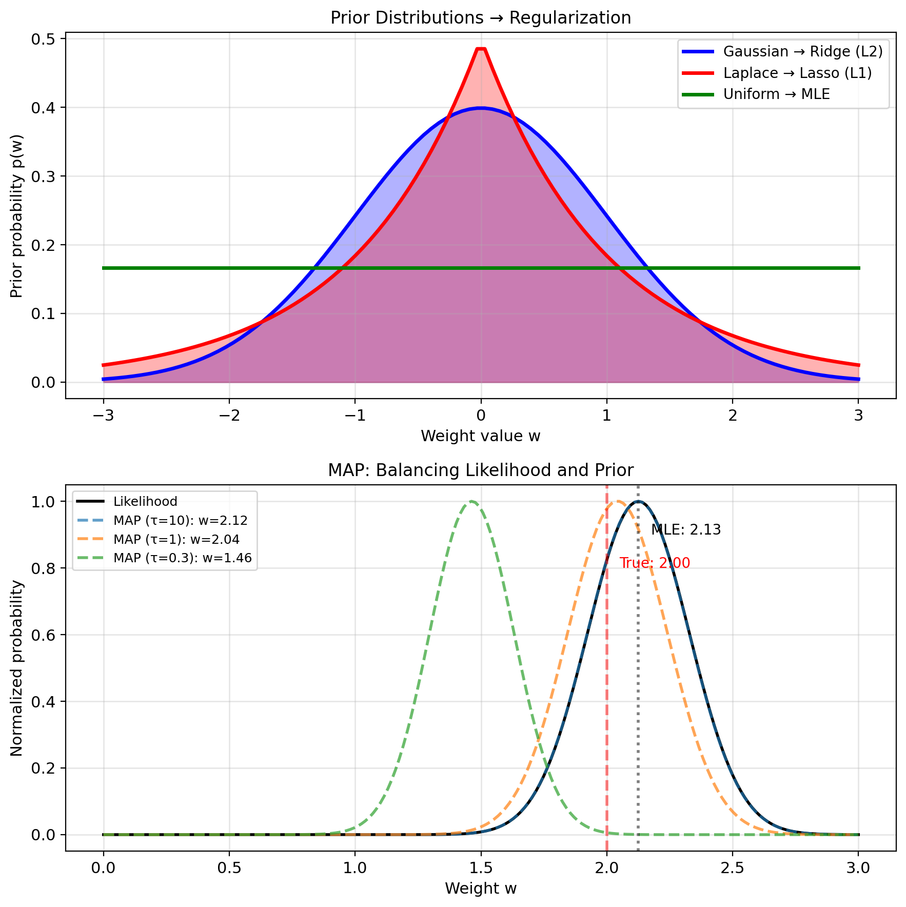
Beyond MLE: Maximum A Posteriori (MAP)
MLE limitation: Ignores prior knowledge
Bayesian approach: Include prior belief \[p(w|\mathcal{D}) \propto p(\mathcal{D}|w) \cdot p(w)\]
MAP estimation: \[\hat{w}_{\text{MAP}} = \arg\max_w p(w|\mathcal{D})\]
Log posterior: \[= \arg\max_w [\log p(\mathcal{D}|w) + \log p(w)]\] \[= \arg\max_w [\text{log-likelihood} + \text{log-prior}]\]
Example: Gaussian prior \(w \sim \mathcal{N}(0, \tau^2 I)\) \[\log p(w) = -\frac{1}{2\tau^2}||w||^2 + \text{const}\]
MAP objective: \[\hat{w}_{\text{MAP}} = \arg\min_w \left[||y - Xw||^2 + \frac{\sigma^2}{\tau^2}||w||^2\right]\]
This is Ridge regression with \(\lambda = \sigma^2/\tau^2\)
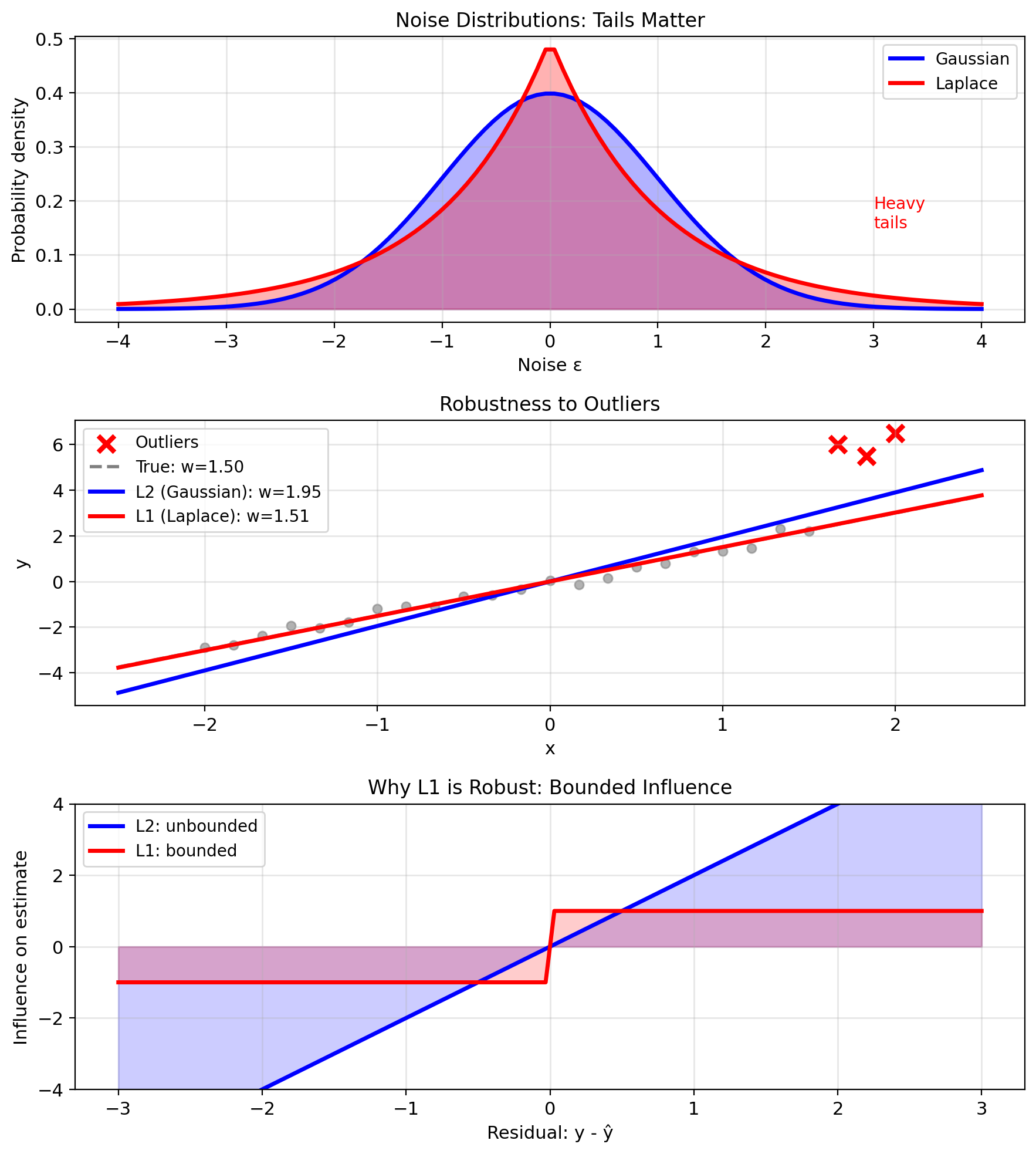
Robust Regression: Laplace Noise → L1 Loss
Why care about different noise models?
Real data often has outliers
- Sensor errors
- Data entry mistakes
- Rare events
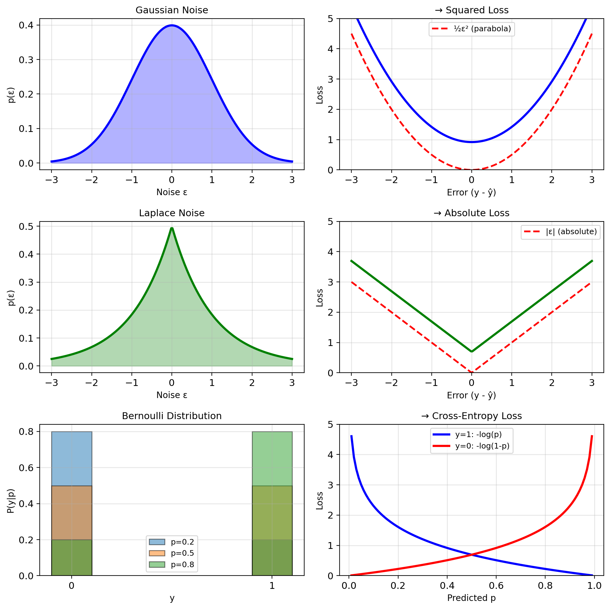
Laplace noise model: \[p(\epsilon) = \frac{1}{2b}\exp\left(-\frac{|\epsilon|}{b}\right)\]
Heavy tails → robust to outliers
Likelihood with Laplace noise: \[p(y|x; w) = \frac{1}{2b}\exp\left(-\frac{|y - w^T x|}{b}\right)\]
Log-likelihood: \[\ell(w) = -n\log(2b) - \frac{1}{b}\sum_{i=1}^n |y_i - w^T x_i|\]
Maximizing \(\ell(w)\) equivalent to minimizing: \[\sum_{i=1}^n |y_i - w^T x_i|\]
L1 loss emerges directly from the Laplace noise assumption.
This is Lasso regression (Least Absolute Shrinkage and Selection Operator).
When Linear Models Need Help
Problem 1: Too many features (\(p > n\))
- \(X^T X\) not invertible
- Infinite solutions
- Which one to choose?
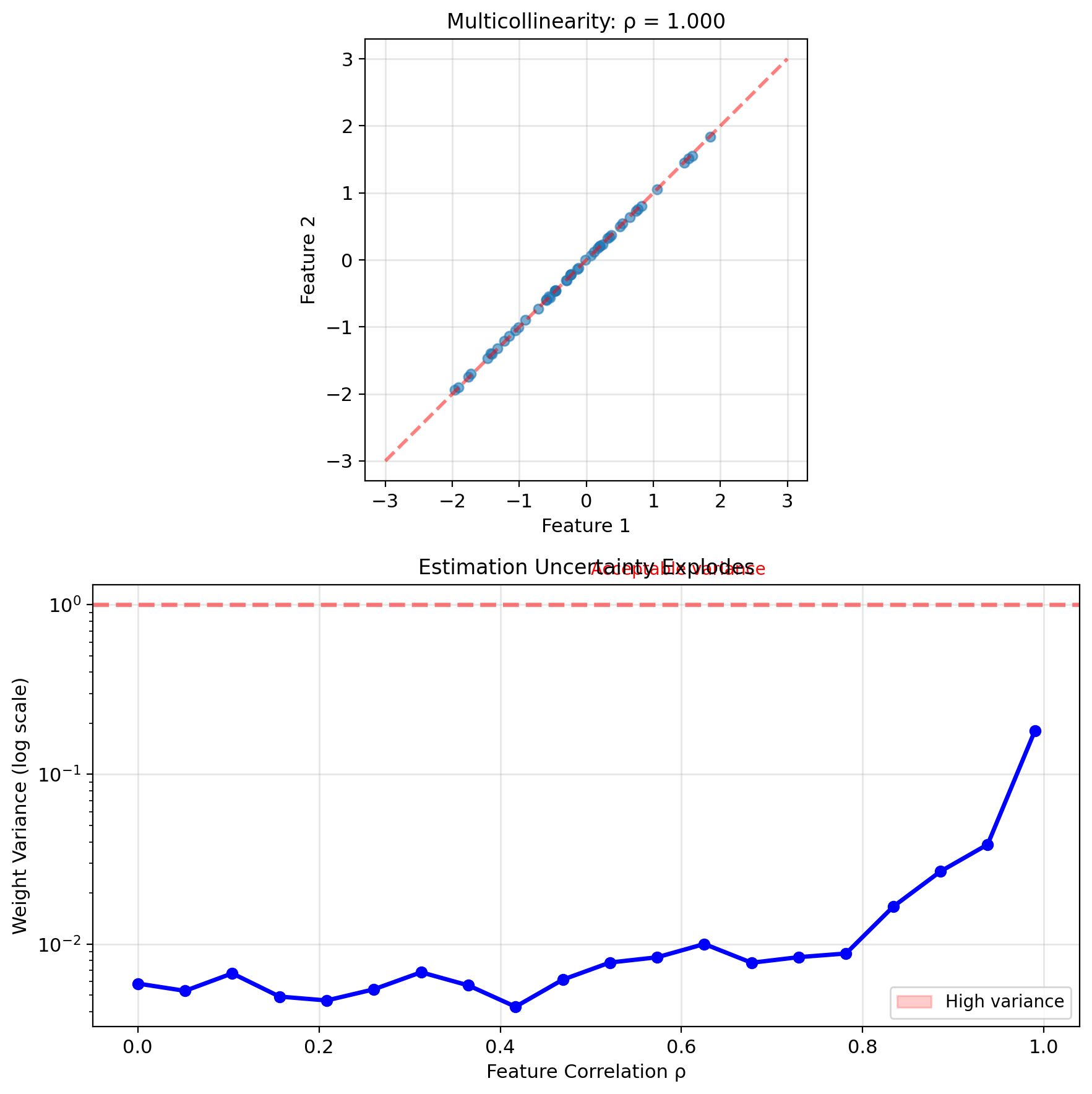
Problem 2: Multicollinearity
- Features highly correlated
- \(X^T X\) nearly singular
- Unstable estimates, huge variance
Problem 3: Overfitting
- Model too flexible
- Memorizes training data
- Poor generalization
Solution approach: Add constraints \[J_{\text{reg}}(w) = ||y - Xw||^2 + \lambda R(w)\]
where \(R(w)\) penalizes complexity
This changes the outcome:
- Unique solution even if \(p > n\)
- Stabilizes estimation
- Controls model complexity
Prediction Error Decomposes into Bias, Variance, and Noise
Setup: \(y = f(x) + \epsilon\), \(\;\mathbb{E}[\epsilon] = 0\), \(\;\text{Var}(\epsilon) = \sigma^2\)
Expand at point \(x_0\), with \(\hat{f}\) random (trained on random data): \[\mathbb{E}[(y - \hat{f}(x_0))^2] = \mathbb{E}[(f(x_0) + \epsilon - \hat{f}(x_0))^2]\]
Independence of \(\epsilon\) and \(\hat{f}\): \[= \mathbb{E}[(f(x_0) - \hat{f}(x_0))^2] + \sigma^2\]
Add and subtract \(\mathbb{E}[\hat{f}(x_0)]\): \[= \text{Var}(\hat{f}(x_0)) + (f(x_0) - \mathbb{E}[\hat{f}(x_0)])^2 + \sigma^2\]
\[\boxed{\text{MSE} = \text{Variance} + \text{Bias}^2 + \sigma^2}\]
For linear models: Variance \(\propto p\sigma^2/n\), bias decreases as \(p\) increases
- \(p\) = number of parameters
- \(n\) = number of samples
Overfitting: Variance dominates bias; training error \(\ll\) test error
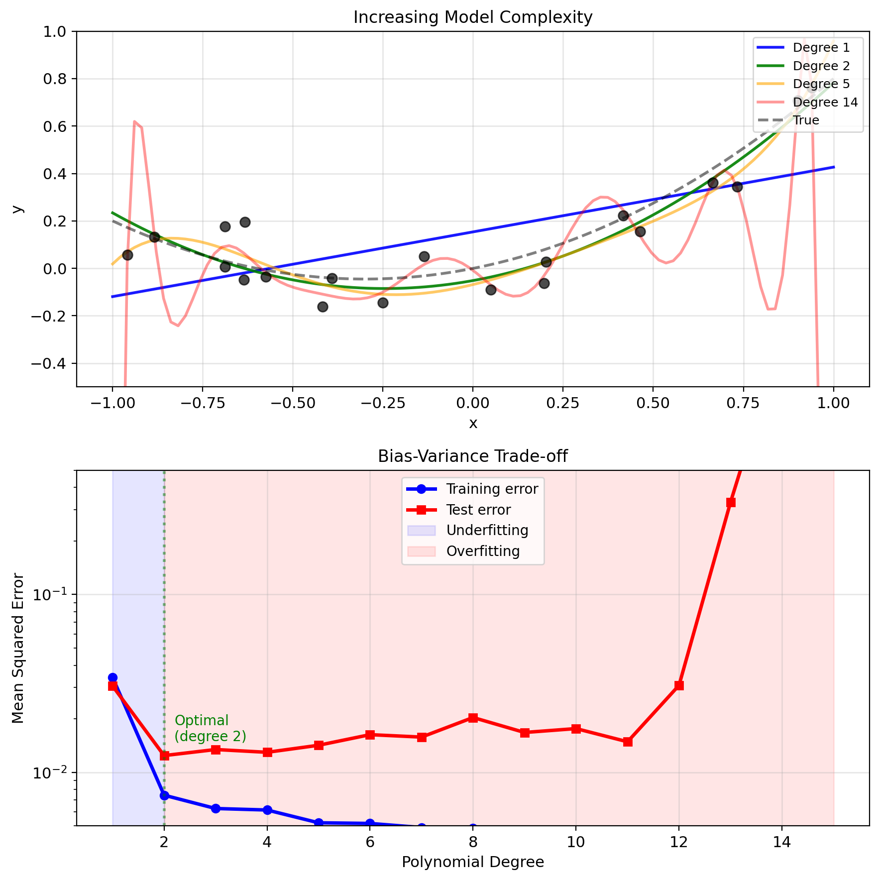
Regularization Controls the Bias-Variance Tradeoff
Evaluation protocol: Split data into training and test sets
- Training error: Loss on data used to fit \(w\)
- Test error: Loss on held-out data, never seen during training
- Overfitting = large gap between training and test error
Concrete example (polynomial regression, \(n=20\), \(\sigma=0.1\)):
| Degree | Bias\(^2\) | Variance | Test MSE |
|---|---|---|---|
| 1 | 0.025 | 0.001 | 0.036 |
| 2 | 0.001 | 0.002 | 0.013 |
| 5 | 0.001 | 0.008 | 0.019 |
| 14 | 0.001 | 0.35 | 0.36 |
Regularization adds a penalty to control variance: \[J_\lambda(w) = \frac{1}{n}\sum_i (y_i - w^T x_i)^2 + \lambda \|w\|^2\]
- \(\lambda = 0\): No penalty → low bias, high variance
- \(\lambda \to \infty\): Heavy penalty → \(w \to 0\) → high bias, zero variance
- Optimal \(\lambda\): Minimizes test error
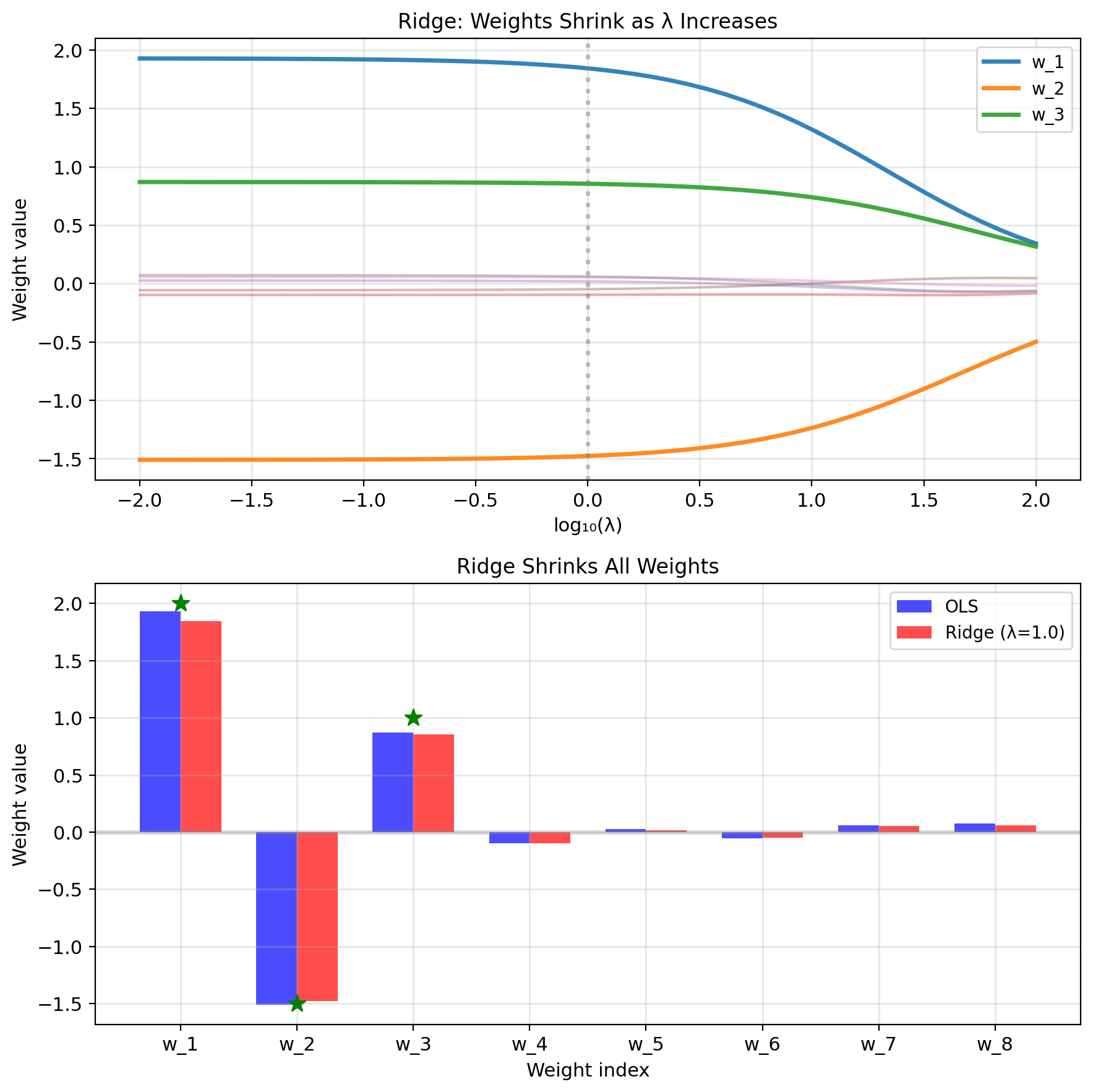
L2 Penalty Guarantees a Unique, Stable Solution
Modified objective: \[J_{\text{reg}}(w) = ||y - Xw||^2 + \lambda ||w||^2\]
Ridge regression: L2 penalty
New solution: \[\hat{w}_{\text{ridge}} = (X^T X + \lambda I)^{-1} X^T y\]
What this does:
- Always invertible (even if \(p > n\))
- Shrinks weights toward zero
- Reduces variance at cost of bias
Bayesian interpretation:
- Prior belief: \(w \sim \mathcal{N}(0, \tau^2 I)\)
- Small weights more likely
- \(\lambda = \sigma^2/\tau^2\)
Connection to MLE:
- MLE: maximize likelihood only
- MAP: maximize posterior \(\propto\) likelihood × prior
- Ridge = MAP with Gaussian prior
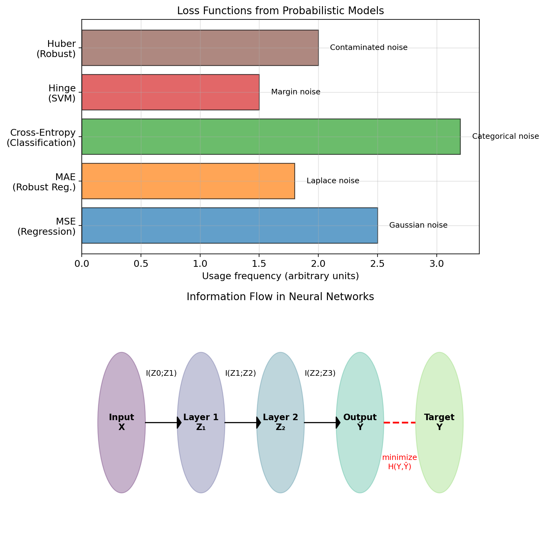
Noise Models Imply Loss Functions
- MLE: Gaussian noise → squared loss
- MLE: Laplace noise → absolute loss
These are specific cases. Information theory provides the general framework:
- Every probabilistic model prescribes a loss function
- Cross-entropy emerges for classification
- KL divergence unifies MLE
- Entropy measures irreducible uncertainty
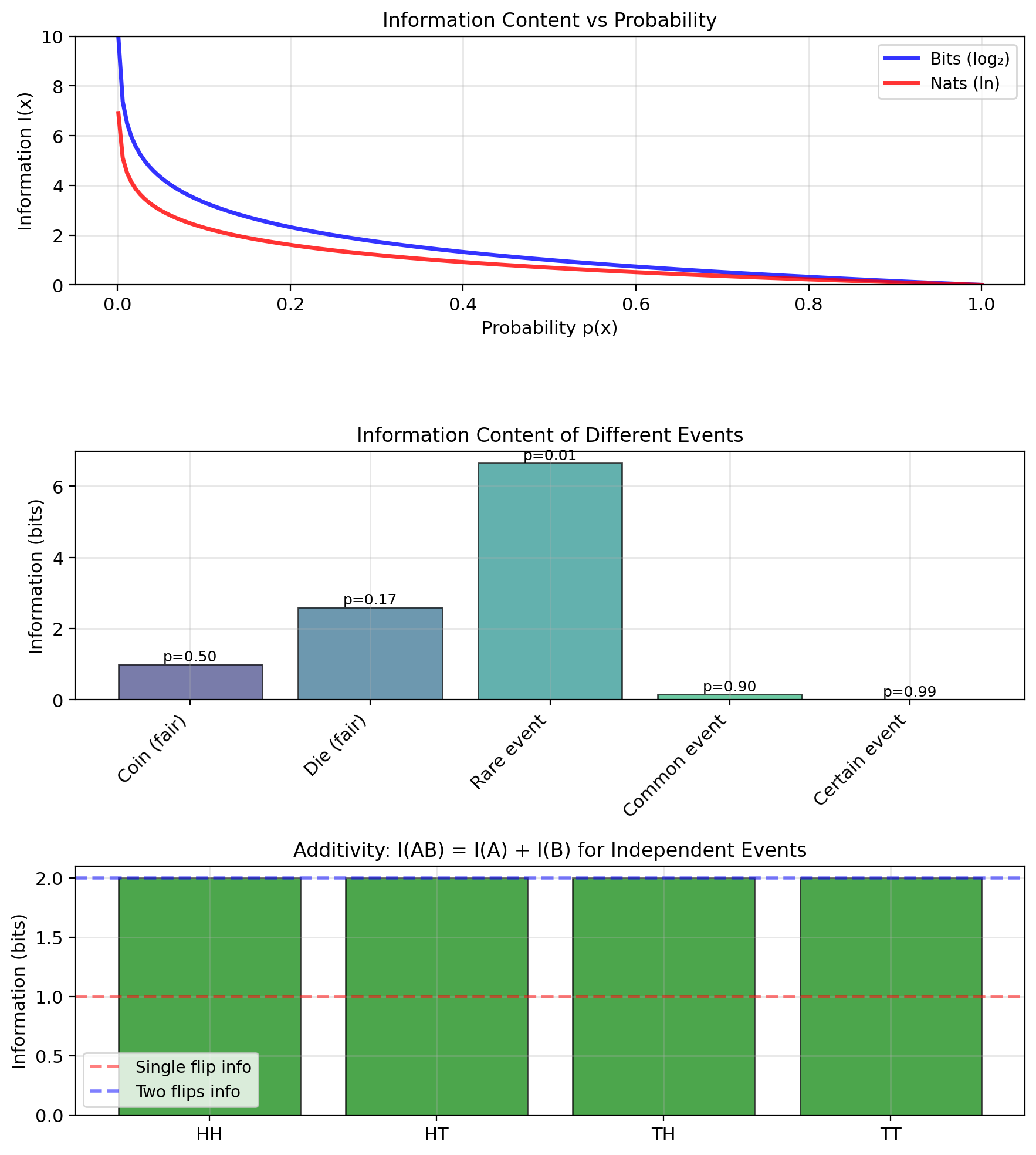
Information Content: Quantifying Surprise
Intuition: Rare events are more “informative”
Information content of a single outcome \(x\): \[I(x) = -\log p(x)\]
Units:
- Base 2: bits (binary digits)
- Base e: nats (natural units)
- Base 10: dits (decimal digits)
Properties:
- \(I(x) \geq 0\) (information is non-negative)
- \(p(x) = 1 \Rightarrow I(x) = 0\) (certain events have no surprise)
- \(p(x) \to 0 \Rightarrow I(x) \to \infty\) (impossible events maximally surprising)
Why logarithm?
- Additivity: Independent events \(A, B\): \[I(A \cap B) = I(A) + I(B)\] \[-\log p(A)p(B) = -\log p(A) - \log p(B)\]
Example: Fair coin flip
- \(p(\text{heads}) = 0.5\)
- \(I(\text{heads}) = -\log_2(0.5) = 1\) bit
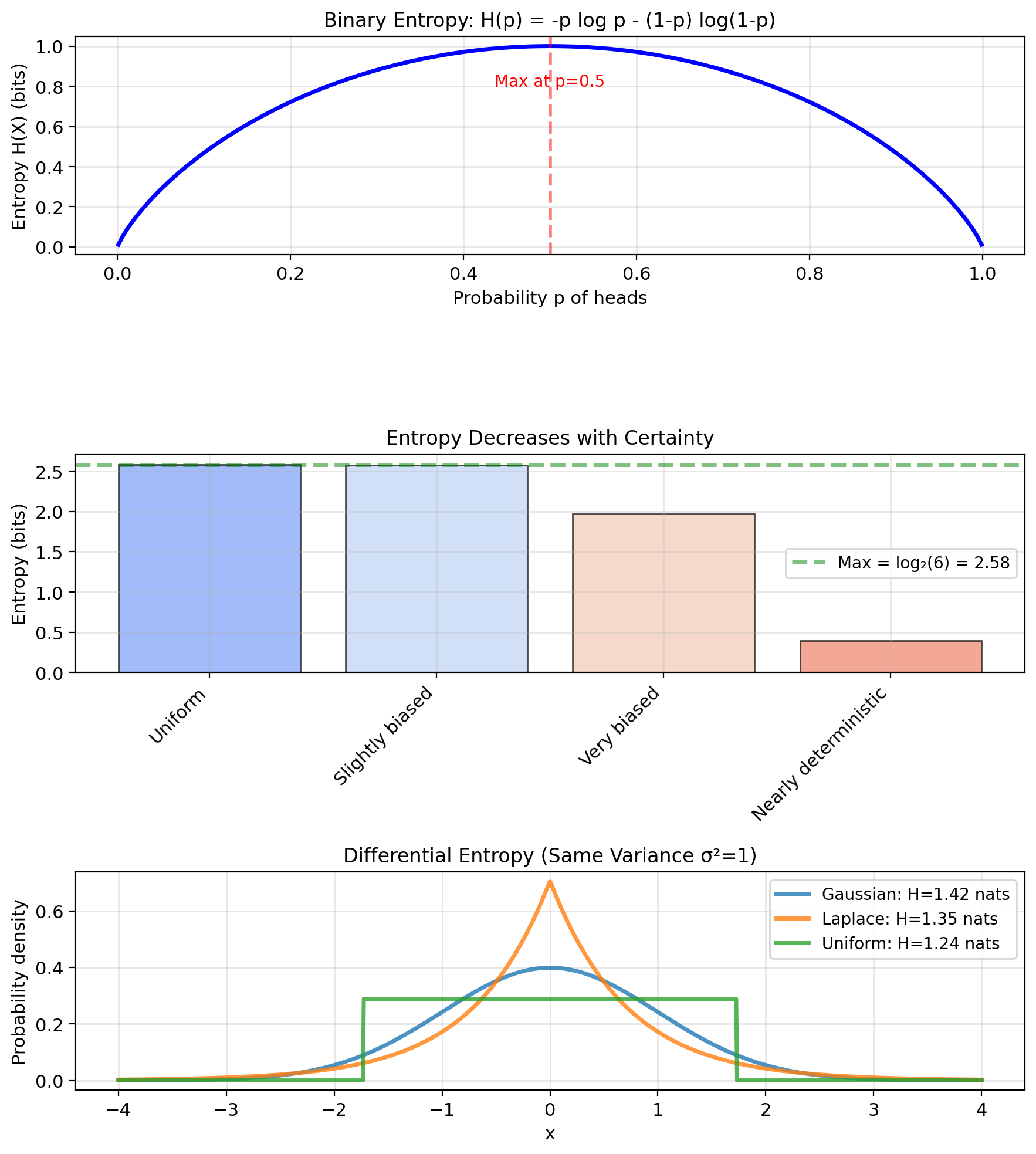
Entropy: Average Information
Entropy = Expected information content across all outcomes \[H(X) = \mathbb{E}[I(X)] = -\mathbb{E}[\log p(X)]\] \[= -\sum_x p(x) \log p(x)\]
Interpretation:
- Average uncertainty before observing \(X\)
- Average surprise when observing \(X\)
- Minimum bits needed to encode \(X\) (on average)
Properties:
- \(H(X) \geq 0\) (entropy is non-negative)
- \(H(X) = 0 \iff X\) is deterministic
- Maximum when uniform: \(H(X) \leq \log |X|\)
Examples:
- Coin (fair): \(H = 1\) bit
- Coin (biased, \(p=0.9\)): \(H = 0.47\) bits
- Die (fair): \(H = \log_2 6 = 2.58\) bits
Continuous case (differential entropy): \[H(X) = -\int p(x) \log p(x) \, dx\]
Note: Can be negative for continuous distributions
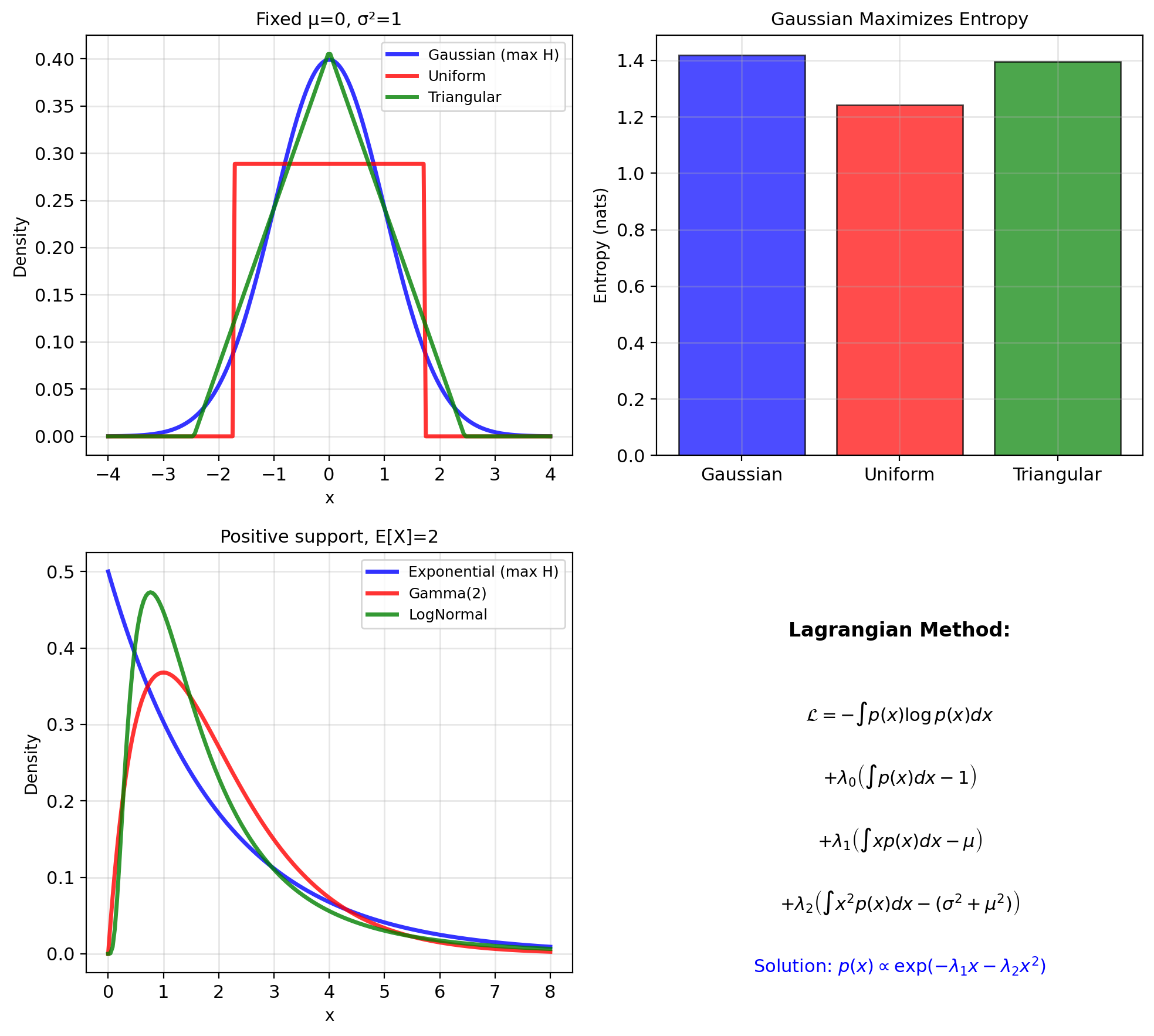
Maximum Entropy Principle
Question: What distribution should we assume given constraints?
Maximum entropy principle: Choose distribution with maximum entropy subject to known constraints
Why?
- Least assumptions beyond constraints
- Most “uncertain” = least biased
- Unique and consistent
Example 1: Known mean and variance \[\max_{p} H(p) \text{ s.t. } \mathbb{E}[X] = \mu, \text{Var}(X) = \sigma^2\]
Solution: Gaussian \(\mathcal{N}(\mu, \sigma^2)\)
Example 2: Positive with known mean \[\max_{p} H(p) \text{ s.t. } X > 0, \mathbb{E}[X] = \lambda\]
Solution: Exponential with rate \(1/\lambda\)
Connection to MLE:
- Gaussian = least informative given fixed mean and variance
- Exponential = least informative for positive data with known mean
- Uniform = least informative with bounded support
Each noise assumption in MLE is the least-informative choice given its constraints.
Lagrangian derivation (Gaussian case): \[\mathcal{L} = -\int p \log p \, dx\] \[+ \lambda_1\!\left(\int x\, p \, dx - \mu\right)\] \[+ \lambda_2\!\left(\int x^2 p \, dx - (\sigma^2 + \mu^2)\right)\] \[\Rightarrow p(x) \propto \exp(-\lambda_1 x - \lambda_2 x^2)\]
Using the Wrong Distribution Has a Cost
Problem: How to measure the difference between two distributions?
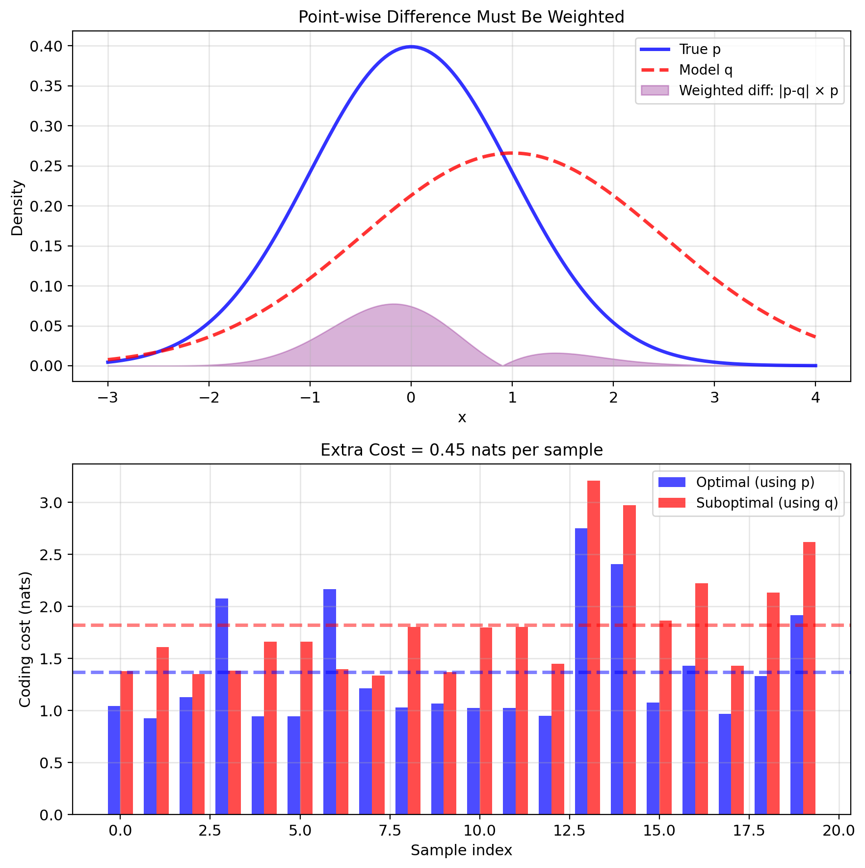
- Not point-wise: distributions are functions
- Need to weight differences by probability
- Want a single scalar measure
Coding perspective: true distribution \(p\), code designed for \(q\)
- Optimal code length for \(x\): \(-\log q(x)\) bits
- Samples actually drawn from \(p\)
- Expected cost: \(\mathbb{E}_p[-\log q(X)]\)
Extra bits from using \(q\) instead of \(p\): \[\underbrace{\mathbb{E}_p[-\log q(X)]}_{H(p,q)} - \underbrace{\mathbb{E}_p[-\log p(X)]}_{H(p)} \geq 0\]
This difference is the KL divergence.
Cross-Entropy Measures Distribution Mismatch
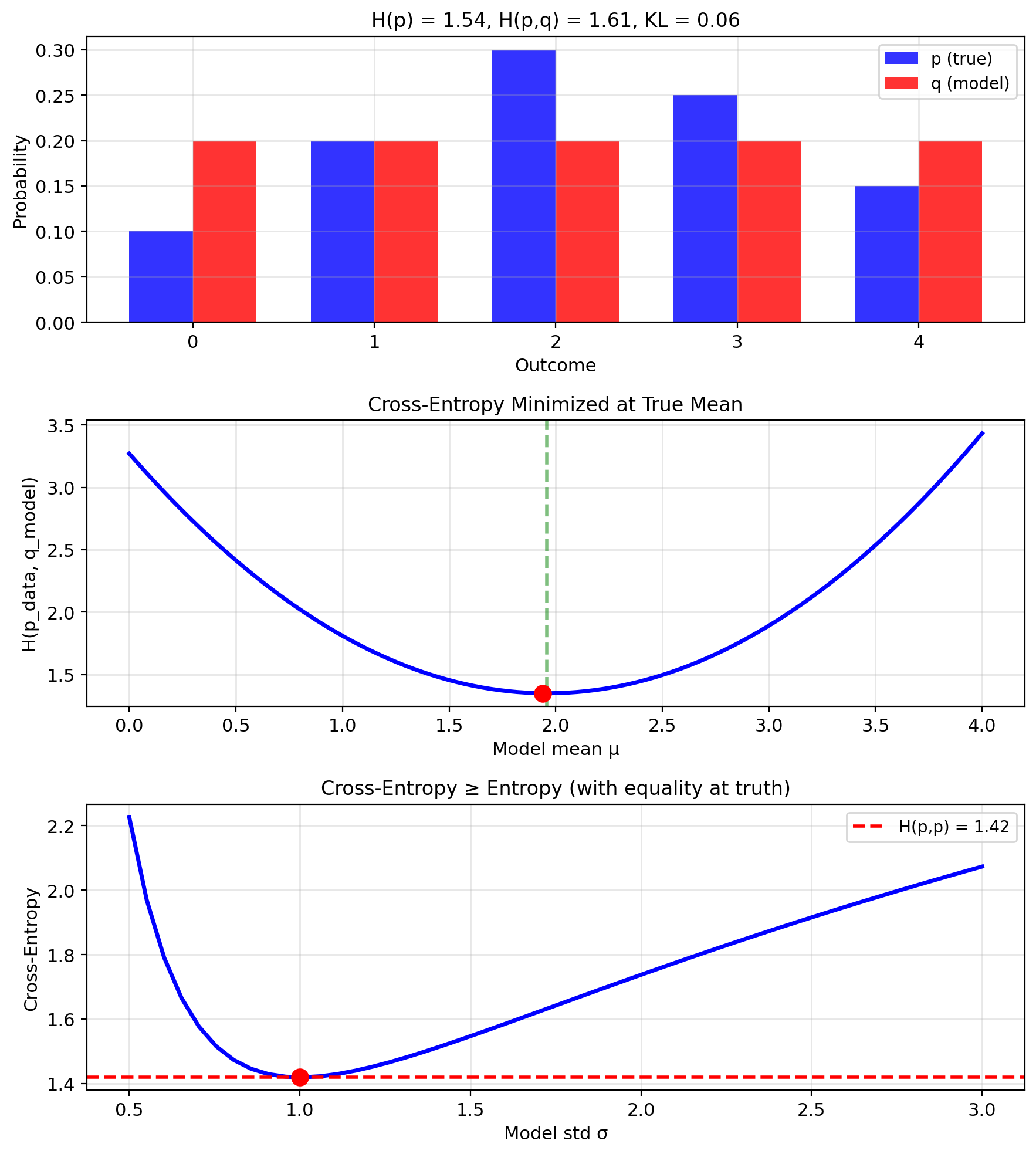
Cross-entropy between \(p\) and \(q\): \[H(p, q) = -\mathbb{E}_p[\log q(X)] = -\int p(x) \log q(x) \, dx\]
Interpretation: Average bits to encode samples from \(p\) using code for \(q\).
- \(H(p, q) \geq H(p)\) (wrong code costs more)
- \(H(p, q) = H(p)\) iff \(p = q\)
- Not symmetric: \(H(p, q) \neq H(q, p)\)
With empirical data \(p_{data} = \frac{1}{n}\sum_{i=1}^n \delta(x - x_i)\):
\[H(p_{data}, q) = -\frac{1}{n}\sum_{i=1}^n \log q(x_i)\]
This is negative average log-likelihood.
KL Divergence: Measuring Distribution Distance
Kullback-Leibler (KL) divergence: \[D_{KL}(p||q) = \mathbb{E}_p\left[\log \frac{p(X)}{q(X)}\right]\] \[= \int p(x) \log \frac{p(x)}{q(x)} \, dx\]
Interpretation:
- Extra bits needed to encode \(p\) using code for \(q\)
- Information lost when approximating \(p\) with \(q\)
- Expected log-likelihood ratio
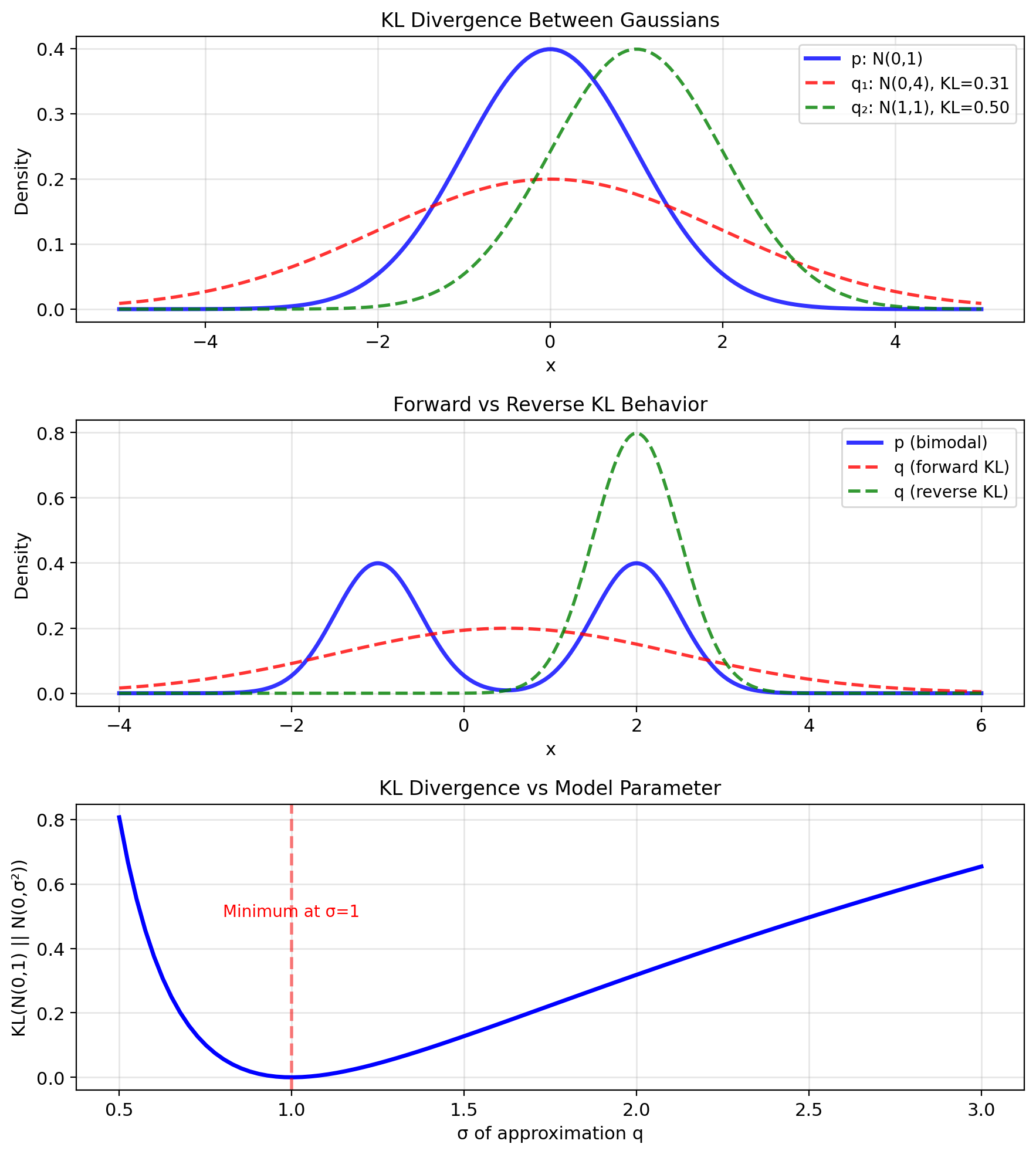
Properties:
- \(D_{KL}(p||q) \geq 0\) (non-negative)
- \(D_{KL}(p||q) = 0 \iff p = q\) a.e.
- Not symmetric: \(D_{KL}(p||q) \neq D_{KL}(q||p)\)
- Not a metric: No triangle inequality
Forward vs Reverse KL:
- Forward \(D_{KL}(p||q)\): \(q\) must cover all of \(p\)
- Reverse \(D_{KL}(q||p)\): \(q\) can be more focused
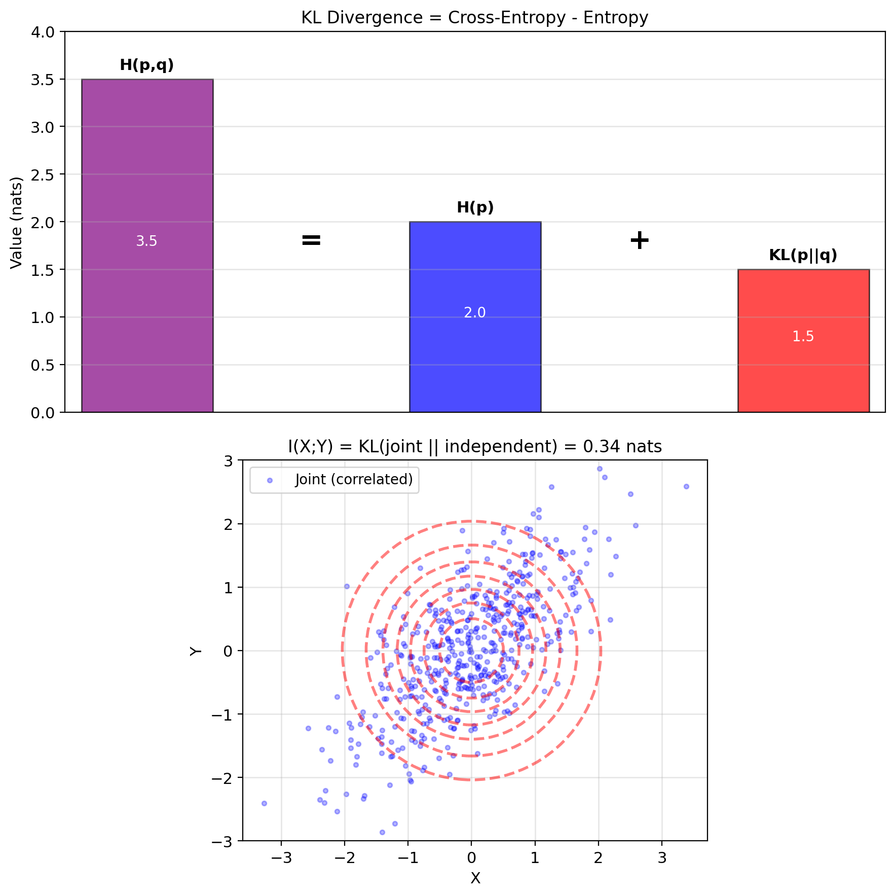
Decomposition (expand the log): \[D_{KL}(p||q) = \int p(x) \log p(x) \, dx - \int p(x) \log q(x) \, dx\] \[= -H(p) + H(p, q)\]
Equivalently: \(H(p, q) = H(p) + D_{KL}(p||q)\)
Connection to likelihood: \[D_{KL}(p_{data}||p_{model}) = \text{const} - \mathbb{E}_{data}[\log p_{model}]\]
Cross-Entropy Decomposes into Entropy Plus KL Divergence
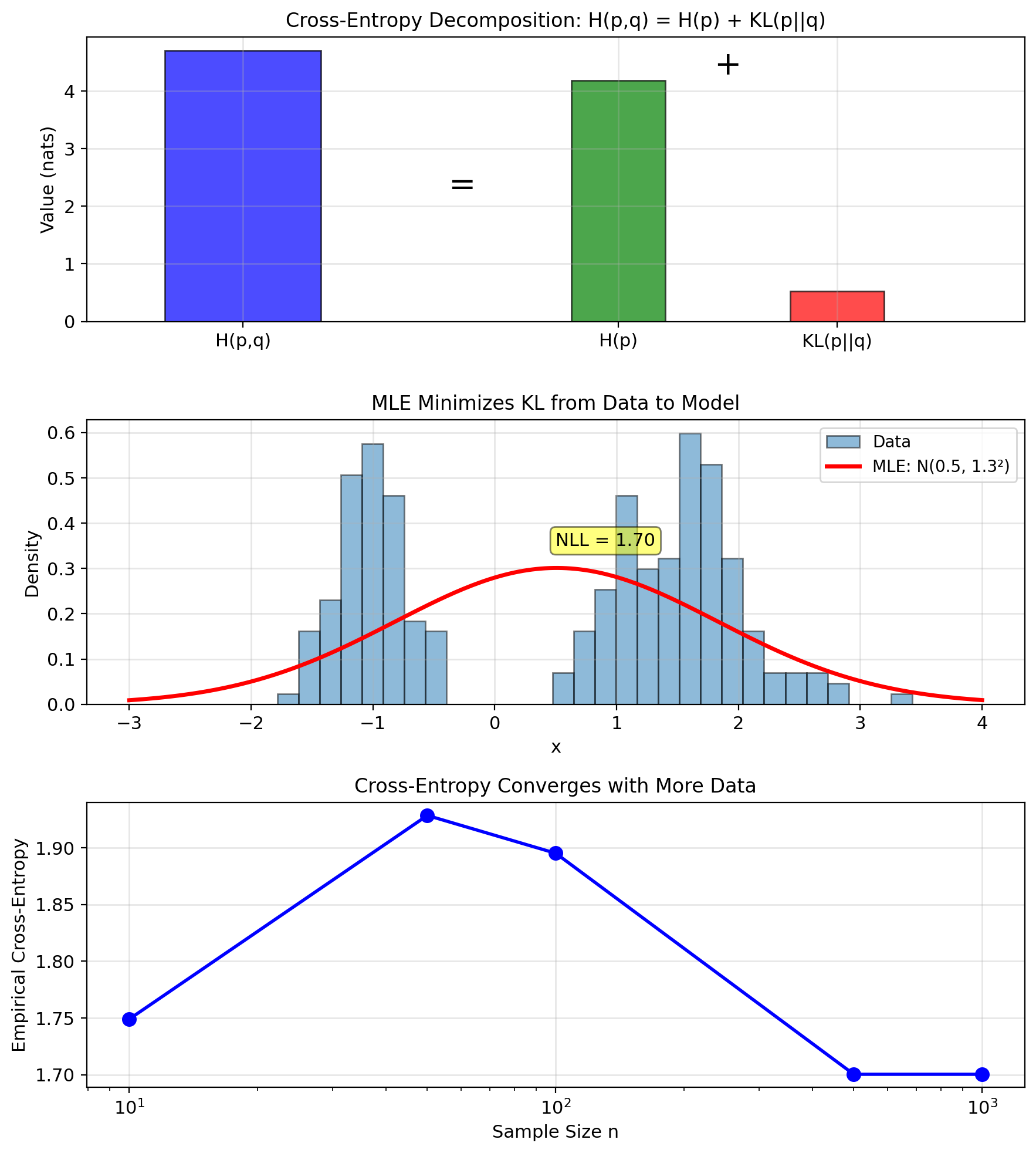
Decomposing KL divergence: \[D_{KL}(p||q) = \int p(x) \log \frac{p(x)}{q(x)} dx\]
Expanding the logarithm: \[D_{KL}(p||q) = \int p(x) \log p(x) dx - \int p(x) \log q(x) dx\] \[= -H(p) + [-\mathbb{E}_p[\log q]]\] \[= H(p, q) - H(p)\]
Decomposition: KL = Cross-entropy - Entropy
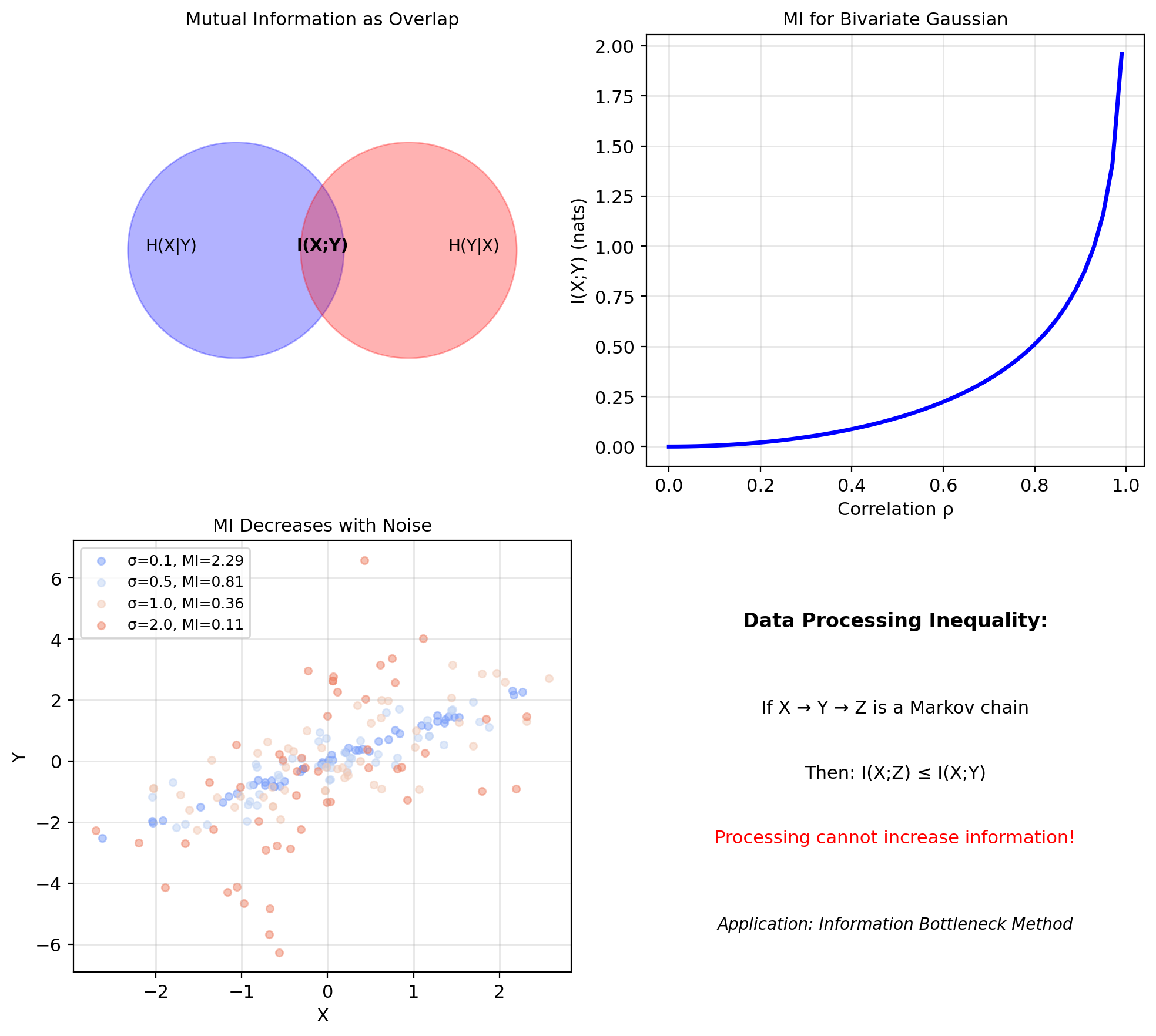
Mutual information is KL of a special form: \[I(X;Y) = D_{KL}\left(p(x,y) \,||\, p(x)p(y)\right)\]
Compares joint distribution to what it would be if independent
- If \(X \perp Y\): \(p(x,y) = p(x)p(y)\) → \(I(X;Y) = 0\)
- If dependent: \(I(X;Y) > 0\) quantifies dependence
Alternative forms: \[I(X;Y) = H(X) - H(X|Y) = H(Y) - H(Y|X)\] \[= H(X) + H(Y) - H(X,Y)\]
Maximum Likelihood via Cross-Entropy Minimization
Learning as distribution matching:
Want model \(q_\theta\) to match data distribution \(p_{data}\)
Minimize KL divergence: \[\min_\theta D_{KL}(p_{data} || q_\theta)\]
Expanding KL: \[D_{KL}(p_{data} || q_\theta) = H(p_{data}, q_\theta) - H(p_{data})\]
Since \(H(p_{data})\) doesn’t depend on \(\theta\): \[\min_\theta D_{KL}(p_{data} || q_\theta) \equiv \min_\theta H(p_{data}, q_\theta)\]
With empirical distribution (data as delta functions): \[p_{data} = \frac{1}{n}\sum_{i=1}^n \delta(x - x_i)\]
\[H(p_{data}, q_\theta) = -\frac{1}{n}\sum_{i=1}^n \log q_\theta(x_i)\]
This is negative average log-likelihood.
\[\min_\theta H(p_{data}, q_\theta) \equiv \max_\theta \frac{1}{n}\sum_{i=1}^n \log q_\theta(x_i)\]
MLE = Cross-entropy minimization = KL minimization
From Noise Models to Loss Functions
Principle: Loss = negative log-likelihood \[\text{Loss}(y, \hat{y}) = -\log p(y|\hat{y})\]
Different noise → different loss:
Gaussian noise: \(y = f(x) + \epsilon\), \(\epsilon \sim \mathcal{N}(0, \sigma^2)\) \[p(y|x) = \frac{1}{\sqrt{2\pi\sigma^2}} \exp\left(-\frac{(y - f(x))^2}{2\sigma^2}\right)\] \[-\log p(y|x) = \frac{(y - f(x))^2}{2\sigma^2} + \text{const}\] → Squared loss
Laplace noise: \(\epsilon \sim \text{Laplace}(0, b)\) \[p(y|x) = \frac{1}{2b} \exp\left(-\frac{|y - f(x)|}{b}\right)\] \[-\log p(y|x) = \frac{|y - f(x)|}{b} + \text{const}\] → Absolute loss
Categorical: \(y \in \{1, ..., K\}\), \(p(y=k|x) = \pi_k\) \[-\log p(y|x) = -\log \pi_y\] → Cross-entropy loss
Discrete Targets Lead to Cross-Entropy Loss
Principle: Loss = negative log-likelihood \[\text{Loss}(y, \hat{y}) = -\log p(y|\hat{y})\]
For continuous targets (from MLE):
- Gaussian noise → squared loss
- Laplace noise → absolute loss
For classification (discrete \(y \in \{1, ..., K\}\)):
Model outputs probabilities: \(\pi_k(x) = P(y=k|x)\)
Categorical distribution: \[p(y|x) = \prod_{k=1}^K \pi_k(x)^{\mathbf{1}_{y=k}}\]
Negative log-likelihood: \[-\log p(y|x) = -\sum_{k} \mathbf{1}_{y=k} \log \pi_k\]
One-hot encoding: \(y_k = \mathbf{1}_{y=k}\) \[\Rightarrow \text{Loss} = -\sum_{k} y_k \log \pi_k\]
This is categorical cross-entropy.
Binary case (\(K=2\)): \[\text{Loss} = -y\log \pi - (1-y)\log(1-\pi)\]
Bernoulli leads to binary cross-entropy
Mutual Information Quantifies Statistical Dependence
Mutual information between \(X\) and \(Y\): \[I(X; Y) = D_{KL}(p(x,y) || p(x)p(y))\] \[= \mathbb{E}_{X,Y}\left[\log \frac{p(X,Y)}{p(X)p(Y)}\right]\]
Equivalent forms: \[I(X; Y) = H(X) - H(X|Y) = H(Y) - H(Y|X)\] \[= H(X) + H(Y) - H(X,Y)\]
Interpretation:
- Information gained about \(X\) by observing \(Y\)
- Reduction in uncertainty of \(X\) given \(Y\)
- Measure of dependence (0 iff independent)
Properties:
- \(I(X; Y) \geq 0\) (non-negative)
- \(I(X; Y) = 0 \iff X \perp Y\) (independence)
- \(I(X; Y) = I(Y; X)\) (symmetric)
- \(I(X; X) = H(X)\) (self-information)
Role in ML:
- Feature selection: pick features \(X_j\) maximizing \(I(X_j; Y)\)
- Representation learning: find \(Z = f(X)\) that preserves \(I(Z; Y)\)
- Information bottleneck: compress \(X\) while retaining information about \(Y\)
Data Processing Inequality: If \(X \to Y \to Z\) is a Markov chain, then \(I(X;Z) \leq I(X;Y)\).
Processing cannot increase information.
Can We Use Regression for Classification?
Binary classification problem:
- Input: \(x \in \mathbb{R}^p\)
- Output: \(y \in \{0, 1\}\) or \(y \in \{-1, +1\}\)
Naive approach: Treat as regression
- Encode classes numerically
- Apply linear regression: \(\hat{y} = w^Tx + b\)
- Threshold the output:
- If \(y \in \{0,1\}\): predict 1 if \(\hat{y} > 0.5\)
- If \(y \in \{-1,+1\}\): predict sign(\(\hat{y}\))
This is valid:
- Classes have numeric labels
- Can minimize squared error
- Produces a decision boundary
But, there are problems.
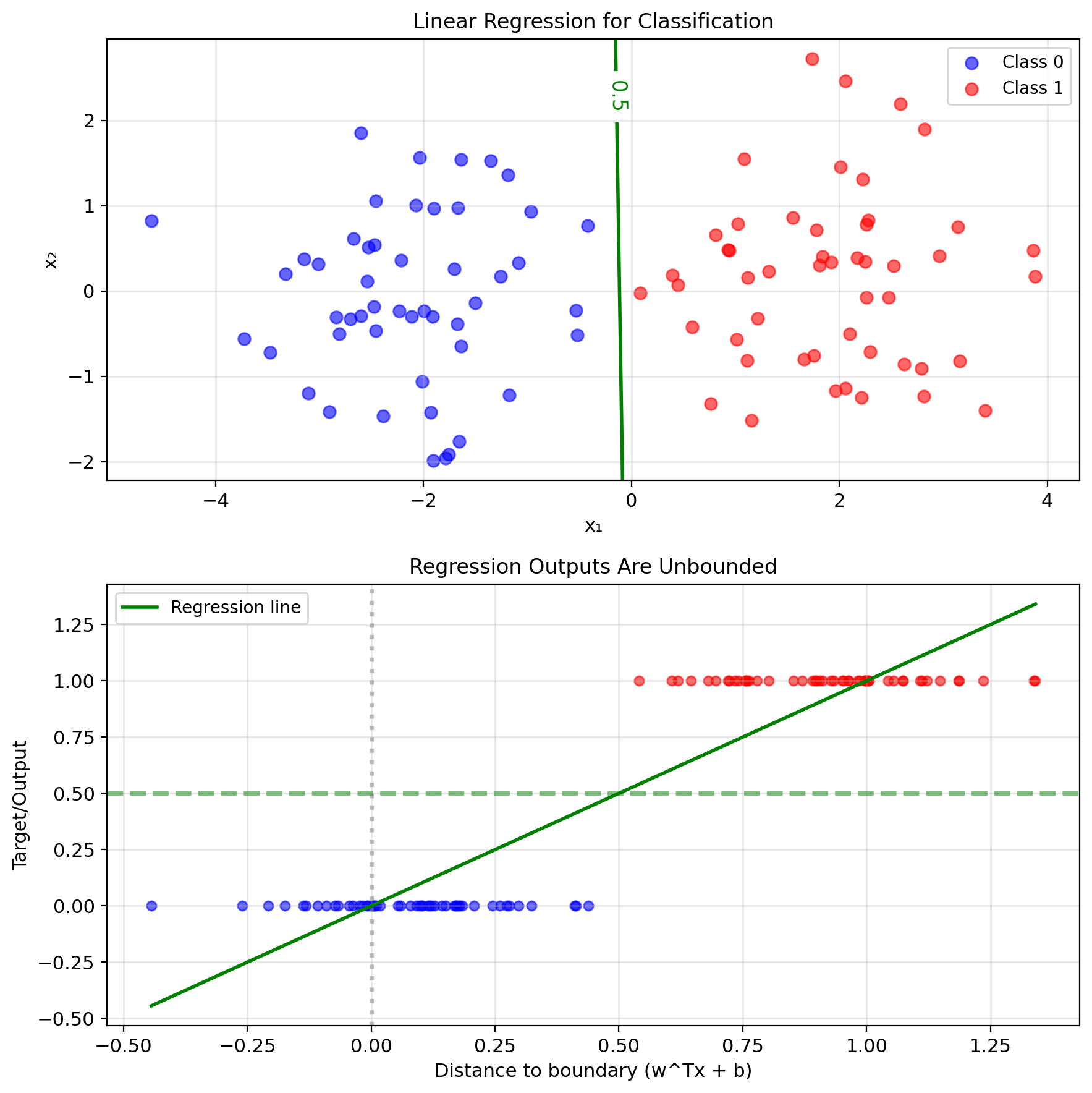
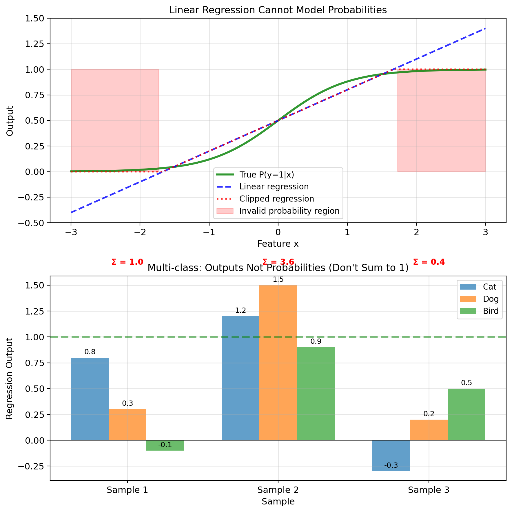
Problem 1: Unbounded Outputs
Regression outputs can be any real number
For points far from boundary:
- \(\hat{y} \gg 1\) or \(\hat{y} \ll 0\)
- Cannot interpret as probability
- \(P(y=1|x) = 2.7\)? Not a valid probability.
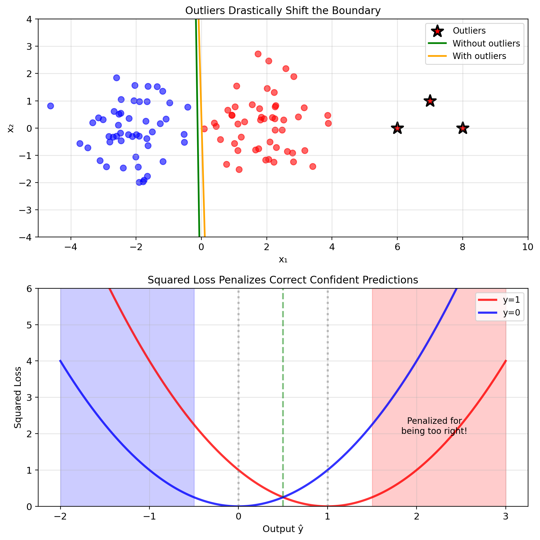
Squared loss biased toward extreme values:
- Point correctly classified at \(\hat{y} = 0.9\)
- Loss = \((1 - 0.9)^2 = 0.01\)
- Point correctly classified at \(\hat{y} = 5.0\)
- Loss = \((1 - 5.0)^2 = 16\) (penalized for being too correct)
Outliers dominate the loss:
- Single point far from boundary
- Contributes enormous squared error
- Pulls decision boundary away from optimal
Need: Output constrained to \([0, 1]\)
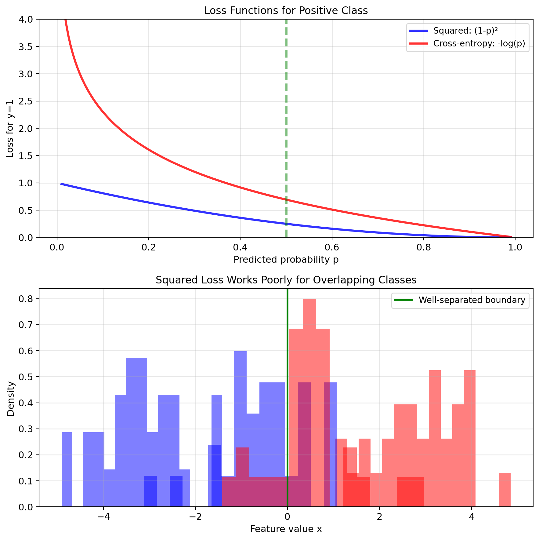
Problem 2: Wrong Loss Function
Classification is fundamentally different from regression
Regression: Minimize distance to target
- Error magnitude matters
- 0.1 error better than 0.2 error
Classification: Correct or incorrect
- Only threshold crossing matters
- Confidence beyond threshold less important
Information theory perspective:
- Binary outcome: \(y \sim \text{Bernoulli}(p)\)
- Optimal loss: \(-y\log p - (1-y)\log(1-p)\)
- Not squared error.
Squared loss for binary data:
- Assumes Gaussian noise
- But \(y \in \{0,1\}\) cannot be Gaussian
- Violates fundamental assumption
The probabilistic model is wrong.
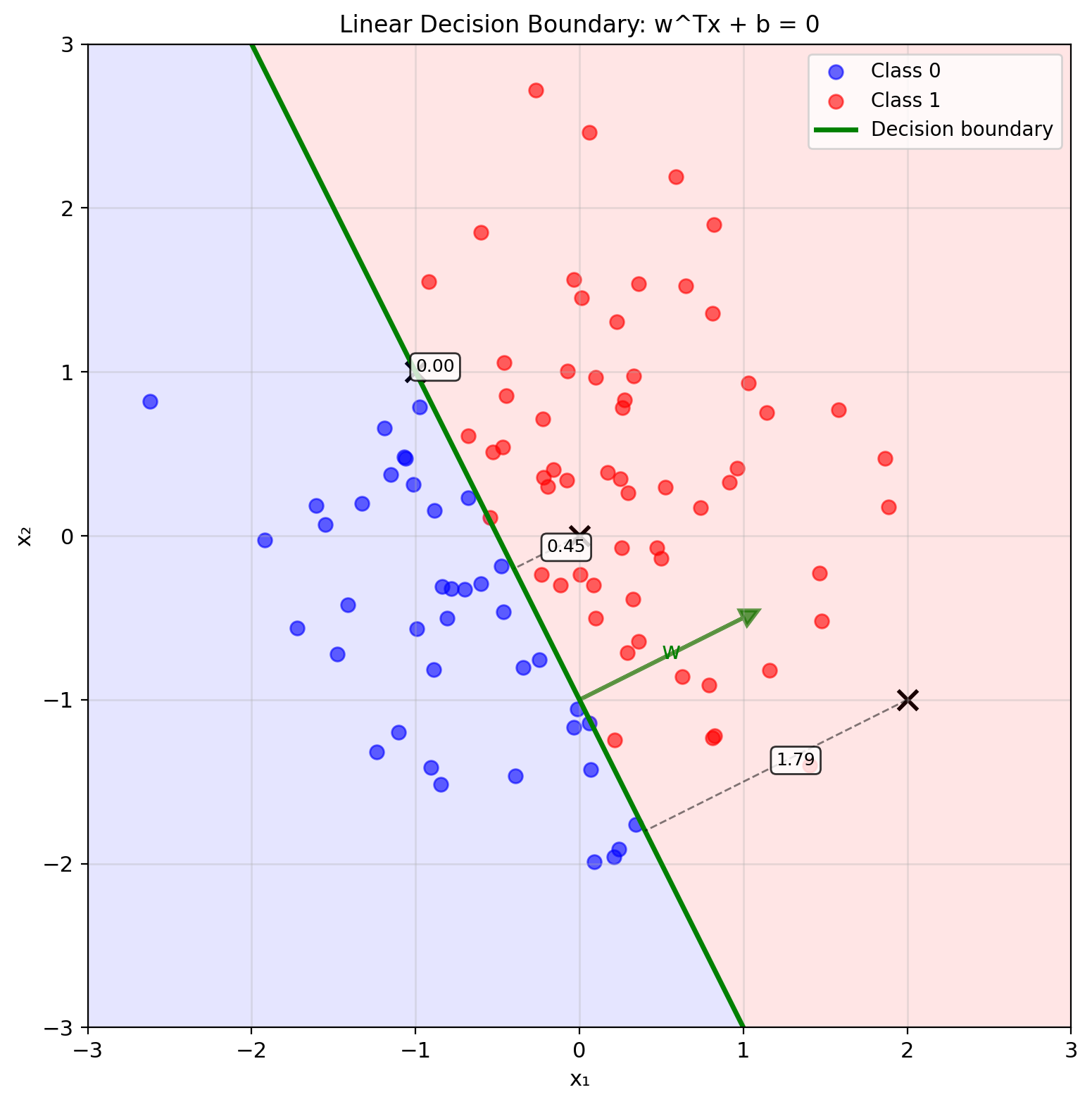
The Separating Hyperplane \(w^Tx + b = 0\)
Linear decision boundary: \[w^Tx + b = 0\]
Defines hyperplane in \(\mathbb{R}^p\)
Geometric interpretation:
- \(w\): normal vector to hyperplane
- \(|b|/||w||\): distance from origin
- Points satisfy: \(w^Tx + b > 0\) (positive side)
- Points satisfy: \(w^Tx + b < 0\) (negative side)
Distance to boundary: \[d(x) = \frac{|w^Tx + b|}{||w||}\]
Signed distance (positive = class 1 side): \[d_{\text{signed}}(x) = \frac{w^Tx + b}{||w||}\]
Decision rule: \[\hat{y} = \begin{cases} 1 & \text{if } w^Tx + b > 0 \\ 0 & \text{if } w^Tx + b \leq 0 \end{cases}\]
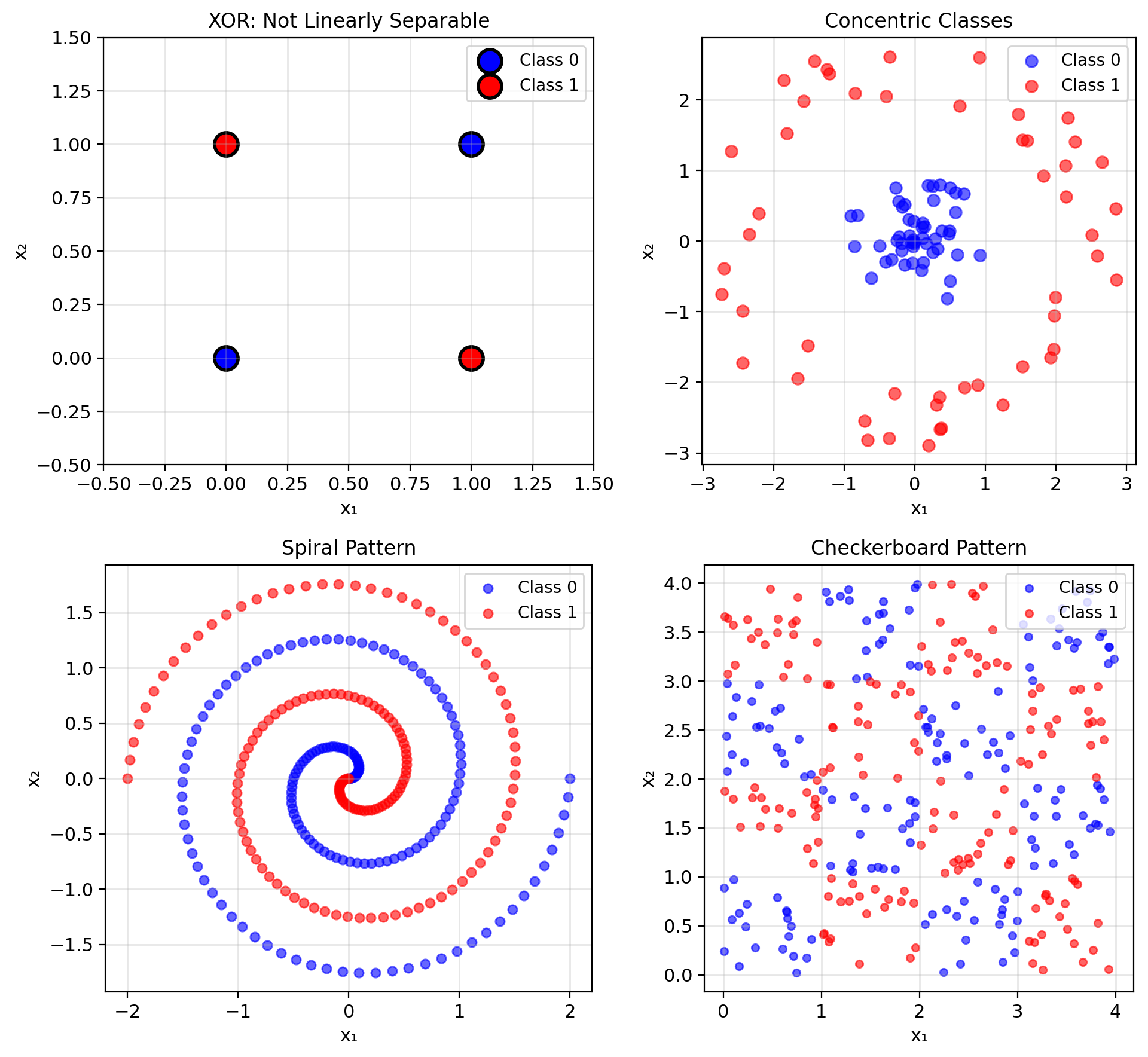
Linear Models Require Linearly Separable Classes
Not all problems are linearly separable
Classic example: XOR
- \((0,0) \to 0\)
- \((0,1) \to 1\)
- \((1,0) \to 1\)
- \((1,1) \to 0\)
No single line can separate the classes.
Linear separability requires: \[\exists w, b : \forall i, \quad y_i(w^Tx_i + b) > 0\]
When linear fails:
- Non-convex class regions
- Classes with holes
- Nested or interleaved patterns
- Manifold structures
Solutions:
- Feature transformation: \(\phi(x)\)
- Multiple linear pieces (neural networks)
- Kernel methods (implicit transformation)
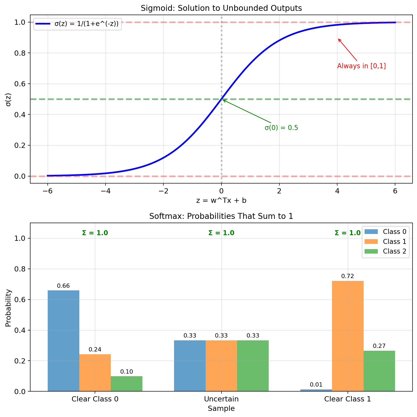
Sigmoid Function Maps \(\mathbb{R} \to (0, 1)\)
Requirements for classification:
- Bounded outputs: Predictions in \([0, 1]\)
- Probabilistic: \(\hat{y} = P(Y=1|x)\)
- Appropriate loss: Penalize confident wrong predictions
The fix: Transform the linear output
\[z = w^T x + b \quad \longrightarrow \quad \sigma(z) = \frac{1}{1+e^{-z}}\]
Sigmoid maps \(\mathbb{R} \to (0, 1)\)
Cross-entropy loss from Bernoulli likelihood:
\[\mathcal{L} = -\frac{1}{n}\sum_{i=1}^n \left[y_i \log \hat{y}_i + (1-y_i)\log(1-\hat{y}_i)\right]\]
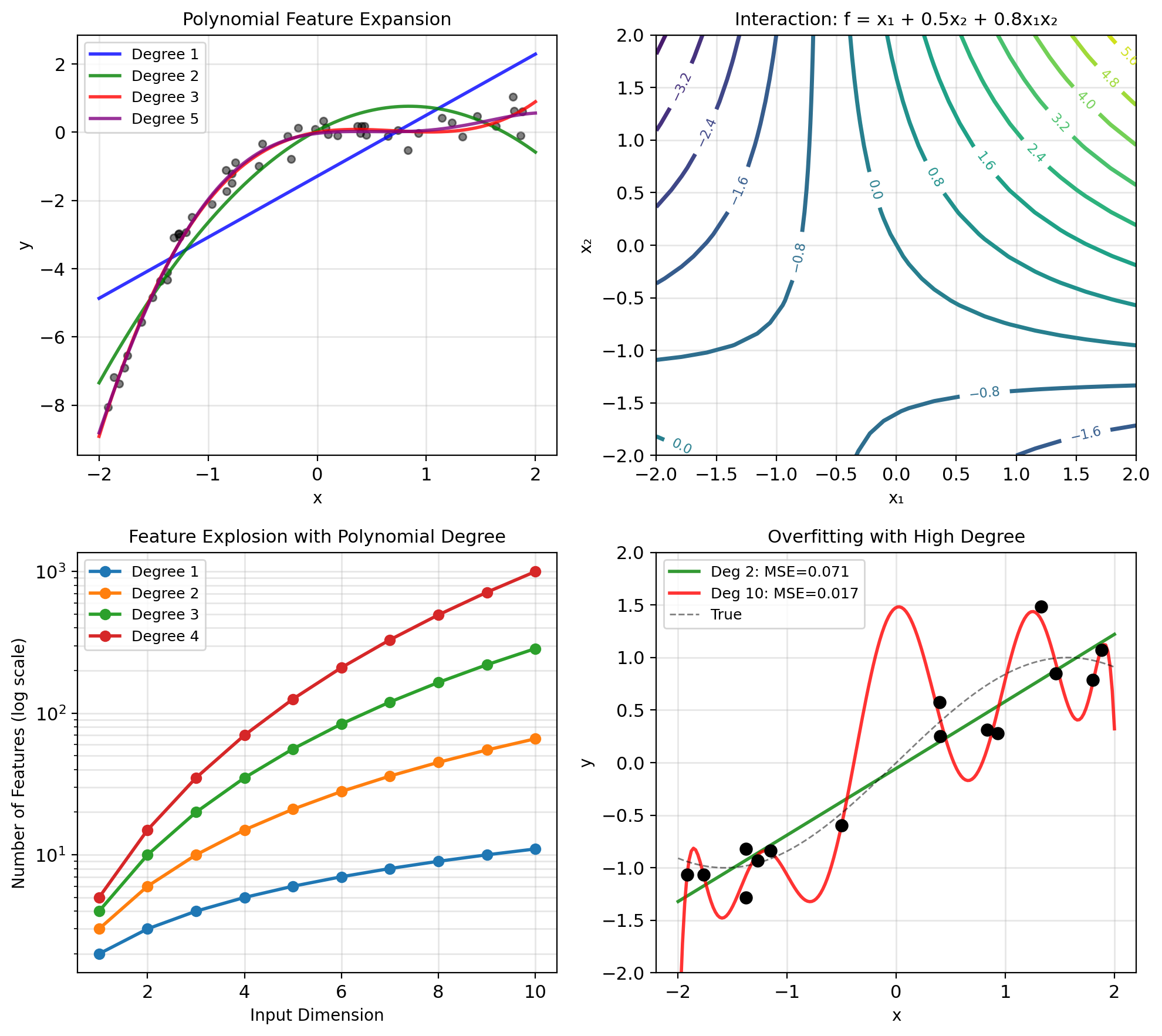
Feature Engineering: Expanding Linear Models
Linear in parameters, not features:
Original features: \(x \in \mathbb{R}^d\)
Transform to: \(\phi(x) \in \mathbb{R}^p\) where \(p > d\)
Model: \(y = w^T\phi(x) + b\)
Polynomial features: \[x \mapsto [1, x, x^2, x^3, ..., x^p]\]
Two variables: \[[x_1, x_2] \mapsto [1, x_1, x_2, x_1^2, x_1x_2, x_2^2, ...]\]
Still solving linear regression: \[\min_w ||\mathbf{y} - \Phi \mathbf{w}||^2\]
where \(\Phi_{ij} = \phi_j(x_i)\)
Complexity growth:
- Degree 2: \(O(d^2)\) features
- Degree 3: \(O(d^3)\) features
- Degree \(p\): \(O(d^p)\) features
This is the curse of dimensionality.
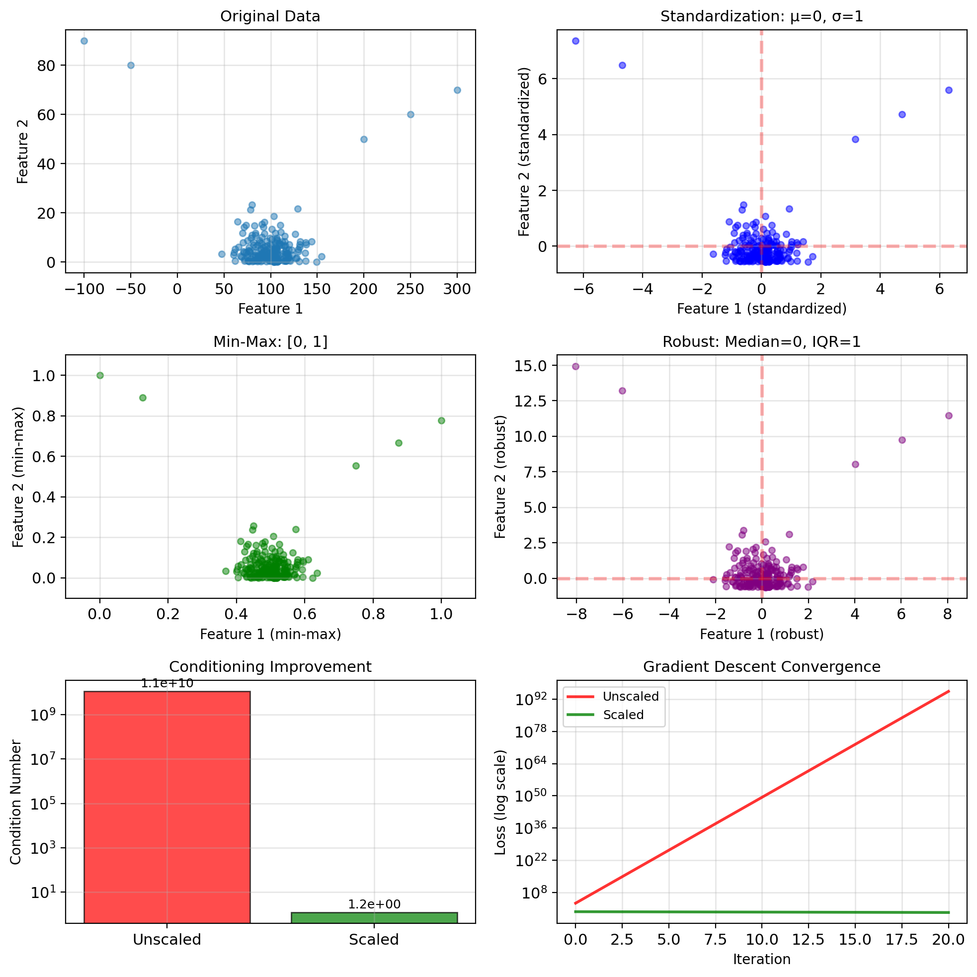
Mismatched Scales Slow Convergence
Why normalize?
- Features on different scales
- Gradient descent convergence
- Numerical stability
Standardization (z-score): \[x' = \frac{x - \mu}{\sigma}\]
- Zero mean, unit variance
- Preserves outliers
- Assumes roughly Gaussian
Min-Max scaling: \[x' = \frac{x - x_{min}}{x_{max} - x_{min}}\]
- Maps to [0, 1]
- Sensitive to outliers
- Bounded output
Robust scaling: \[x' = \frac{x - \text{median}}{\text{IQR}}\]
- Uses median and interquartile range
- Robust to outliers
When to use which:
- Standardization: Most cases, especially with Gaussian assumptions
- Min-Max: Neural networks, bounded inputs needed
- Robust: Data with outliers
Residual Structure Exposes Bad Assumptions
Residuals: \(e_i = y_i - \hat{y}_i\)
Assumptions to check:
Linearity: Residuals vs fitted values
- Should show no pattern
- Curvature suggests nonlinearity
Homoscedasticity: Constant variance
- Residual spread shouldn’t change
- Funnel shape = heteroscedasticity
Normality: Q-Q plot
- Points should follow diagonal
- Heavy tails or skewness problematic
Independence: Autocorrelation
- No pattern in residual sequence
- Durbin-Watson test
When linear regression fails:
- Nonlinear relationships → Polynomial/nonlinear models
- Non-constant variance → Transform response or weighted regression
- Non-normal errors → Robust regression or different loss
- Correlated errors → Time series models
From Normal Equations to np.linalg.solve
NumPy implementation:
# Normal equations
def linear_regression_normal(X, y):
    # Add bias column
    X_b = np.c_[np.ones(len(X)), X]
    # Solve normal equations
    theta = np.linalg.solve(X_b.T @ X_b, X_b.T @ y)
    return theta

# Gradient descent
def linear_regression_gd(X, y, lr=0.01, epochs=1000):
    n, p = X.shape
    X_b = np.c_[np.ones(n), X]
    theta = np.zeros(p + 1)

    for _ in range(epochs):
        gradients = 2/n * X_b.T @ (X_b @ theta - y)
        theta = theta - lr * gradients
return thetaScikit-learn:
from sklearn.linear_model import LinearRegression
model = LinearRegression()
model.fit(X, y)
# Coefficients: model.coef_, model.intercept_
Scikit-learn advantages:
- Handles edge cases
- Built-in preprocessing
- Cross-validation support
- Multiple solver options
\(R^2\): Variance Explained Beyond the Mean
Mean Squared Error (MSE): \[\text{MSE} = \frac{1}{n}\sum_{i=1}^n (y_i - \hat{y}_i)^2\]
Root MSE: \(\text{RMSE} = \sqrt{\text{MSE}}\) (same units as \(y\))
R² (Coefficient of Determination): \[R^2 = 1 - \frac{\text{SS}_{\text{res}}}{\text{SS}_{\text{tot}}} = 1 - \frac{\sum (y_i - \hat{y}_i)^2}{\sum (y_i - \bar{y})^2}\]
- \(R^2 = 1\): Perfect fit
- \(R^2 = 0\): No better than mean
- \(R^2 < 0\): Worse than mean (possible on test set)
Mean Absolute Error (MAE): \[\text{MAE} = \frac{1}{n}\sum_{i=1}^n |y_i - \hat{y}_i|\]
More robust to outliers than MSE
Classification metrics (linear as classifier):
- Accuracy: Fraction correct
- Confusion matrix
- But linear regression is poorly suited for classification.