Training Deep Networks
EE 541 - Unit 7A
Deeper Networks Are More Accurate at Equal Parameter Count
Task: transcribing multi-digit house numbers from Street View photographs (Goodfellow et al. 2014)
Three families, each grown by adding parameters to some of its layers
- \(3\) layers, wider convolutional layers (blue): highest at \(93.2\%\) near \(17\) million parameters
- \(3\) layers, wider fully connected layers (green): near \(93\%\) from \(32\) to \(81\) million
- \(11\) layers (red): \(95.2\%\) at \(16\) million, \(96.0\%\) at \(55\) million
At about \(16\) million parameters: \(95.2\%\) with \(11\) layers, \(93.2\%\) with \(3\)
More parameters can lower accuracy: both \(3\)-layer curves fall past about \(20\) million, which the book attributes to overfitting
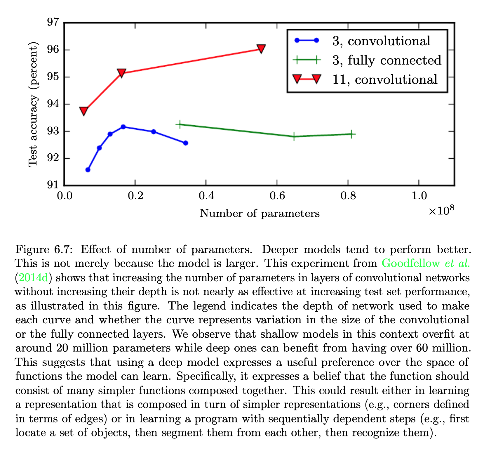
Goodfellow, Bengio, Courville, Deep Learning, Fig. 6.7
Deep Networks Compose Layer Functions
Layer \(l\): \(f^{(l)}(\mathbf{a}) = \sigma^{(l)}\big(\mathbf{W}^{(l)}\mathbf{a} + \mathbf{b}^{(l)}\big)\), \(\;\mathbf{W}^{(l)} \in \mathbb{R}^{n_l \times n_{l-1}}\), \(\;n_l n_{l-1} + n_l\) parameters
\(L\) layers, \(L - 1\) of them hidden:
\[\hat{\mathbf{y}} = f^{(L)}\Big(f^{(L-1)}\big(\cdots f^{(1)}(\mathbf{x})\cdots\big)\Big)\]
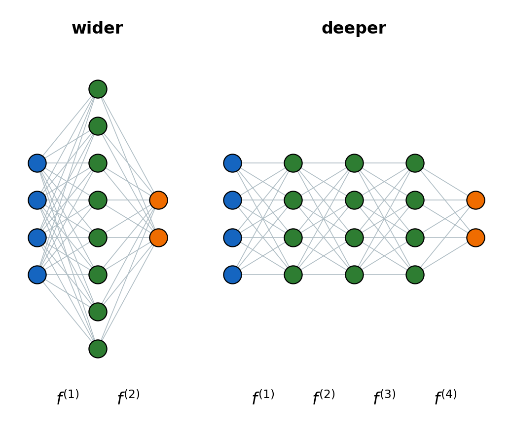
Two ways to grow a network (figure)
- Wider: more units in a layer, all computed from the same input
- Deeper: one more function, applied to the previous layer’s output
Equal parameter count, \(784\) inputs and \(10\) classes, \(269{,}322\) parameters: one hidden layer of \(339\) units, two of \(256\), four of \(195\), or eight of \(147\)
- The first layer’s \(785\, n_1\) parameters are \(99\%\) of the count with one hidden layer, \(43\%\) with eight
Deeper Layers Separate Class Distributions
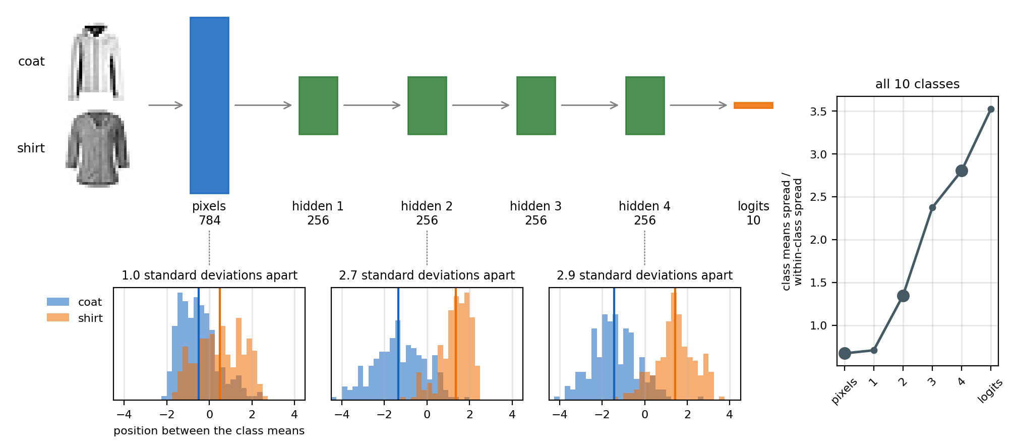
Network: four hidden ReLU layers of \(256\) units, trained on FashionMNIST, \(88.7\%\) test accuracy
Measured on \(2{,}000\) test images
- Histograms: coat and shirt images on the line through their two class means
- Right: spread of all \(10\) class means over the spread within a class
\(\mathrm{MSE}\) = Noise Variance + Approximation Error
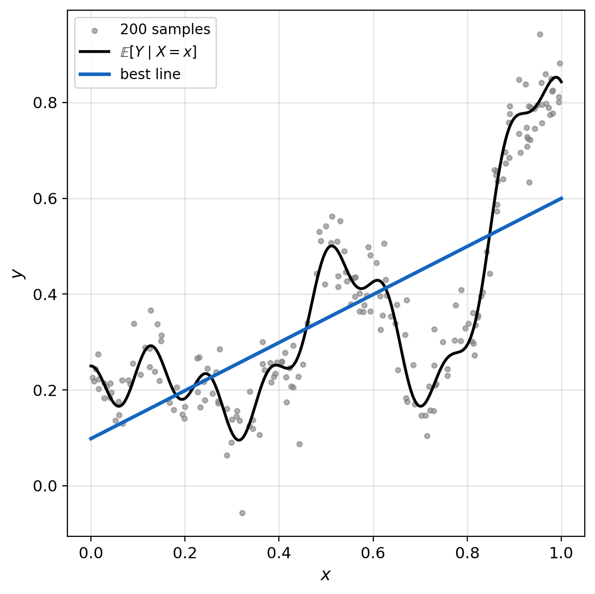
Regression function \(\mathbb{E}[Y \mid X = x]\): the MMSE predictor
Any predictor \(f\), under squared loss:
\[\mathrm{MSE}(f) = \mathbb{E}[\mathrm{Var}(Y \mid X)] + \mathbb{E}\big[(f(X) - \mathbb{E}[Y \mid X])^2\big]\]
Model class \(\mathcal{F}\), with best member \(f^*\): the approximation error is the second term at \(f^*\)
- Zero only if \(\mathbb{E}[Y \mid X = x]\) is in \(\mathcal{F}\)
- More samples estimate \(f^*\) better and leave its error unchanged
Example (figure): \(g(x) = 0.2 + 0.4x^2 + 0.3x \sin 15x + 0.05 \cos 50x\), \(X\) uniform on \([0, 1]\), noise standard deviation \(0.05\)
- Best line: \(0.0225 = 0.0025\) noise \(+\ 0.020\) approximation error
The Staircase Error Vanishes as \(\Delta \to 0\)
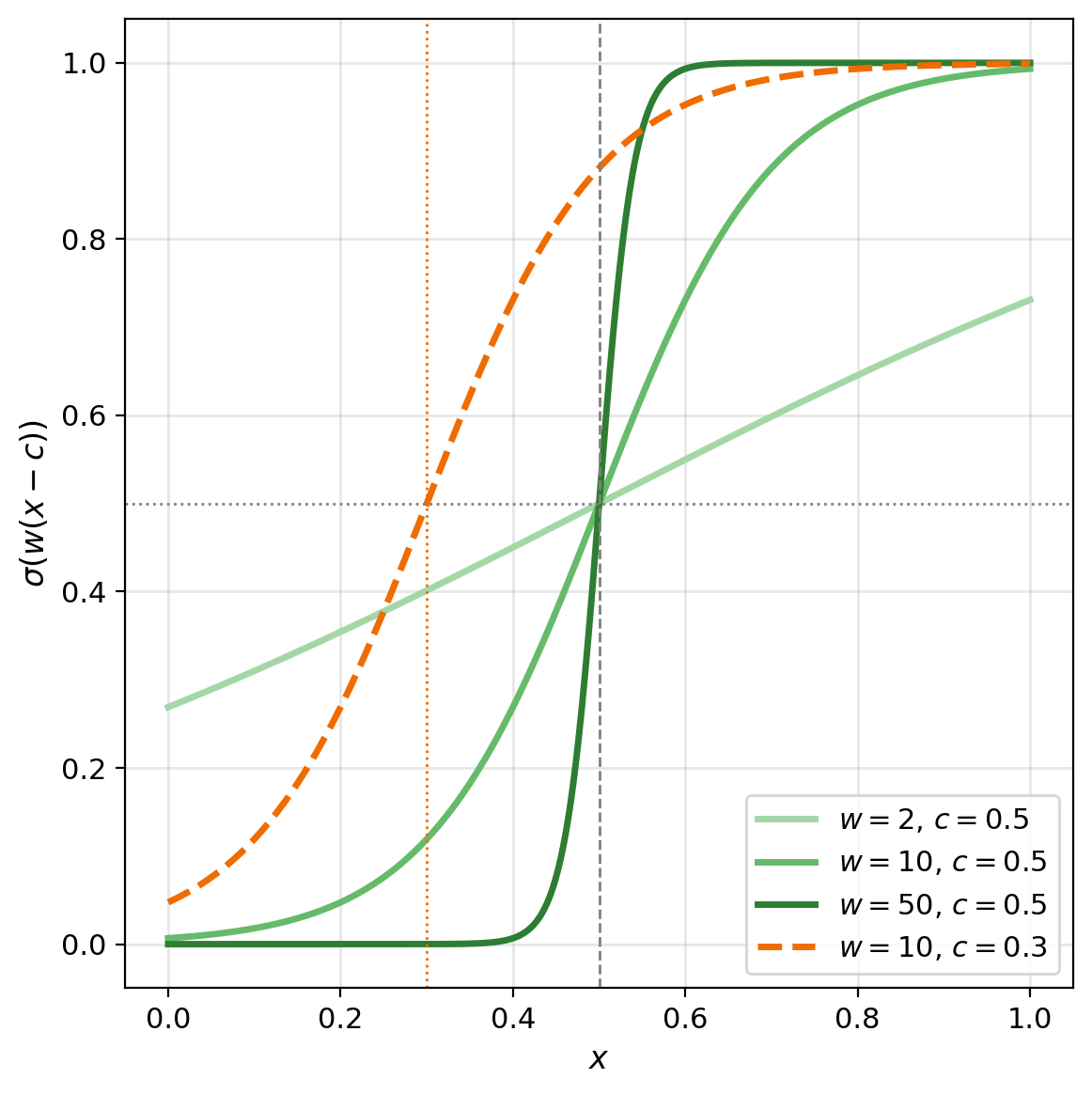
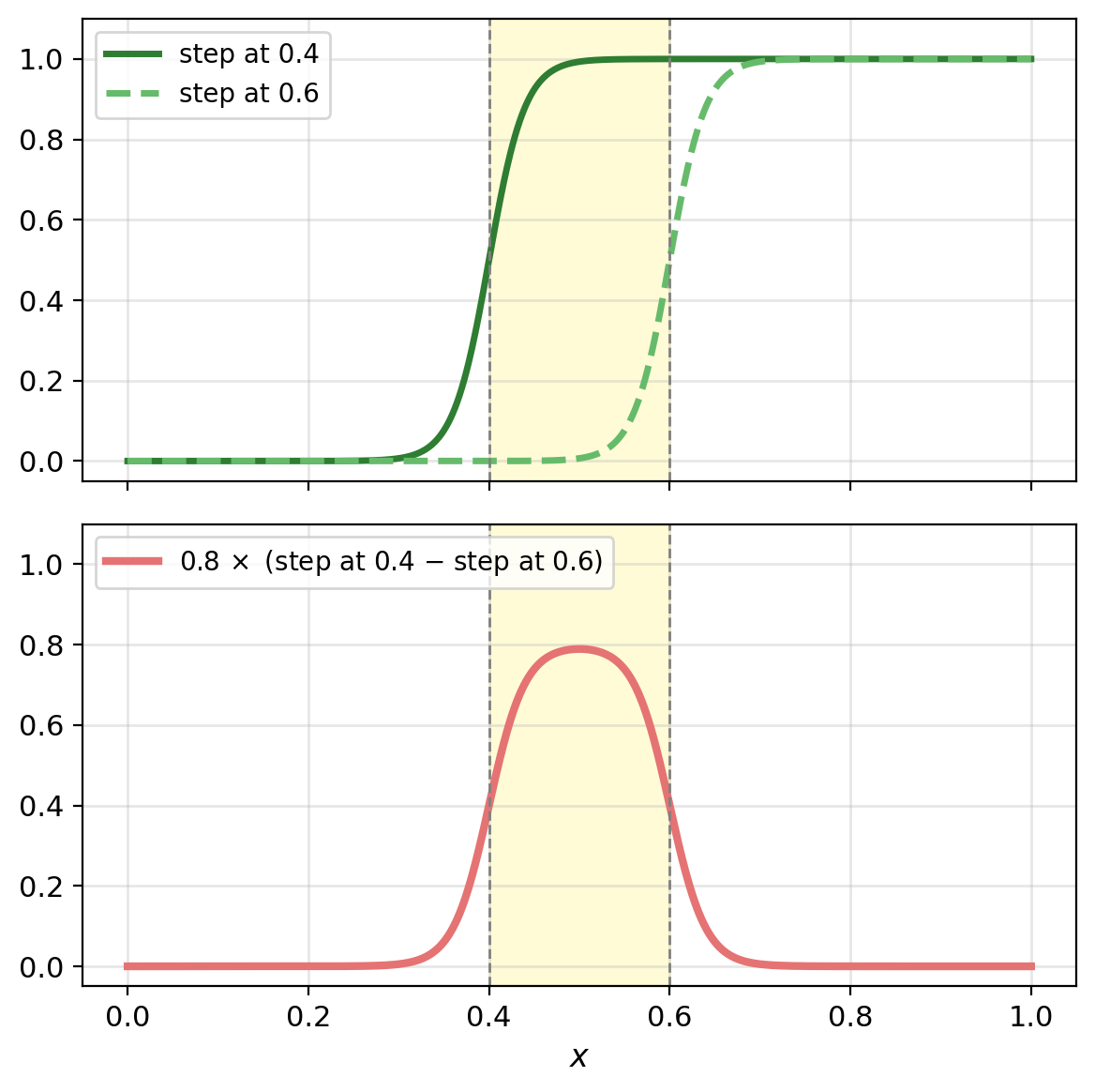
Construction for one input: \([0, 1]\) cut into cells of width \(\Delta\), one bump per cell with height \(g\) at the cell’s center
- \(2/\Delta\) hidden units in one hidden layer
- The sum is a staircase \(h_\Delta\)
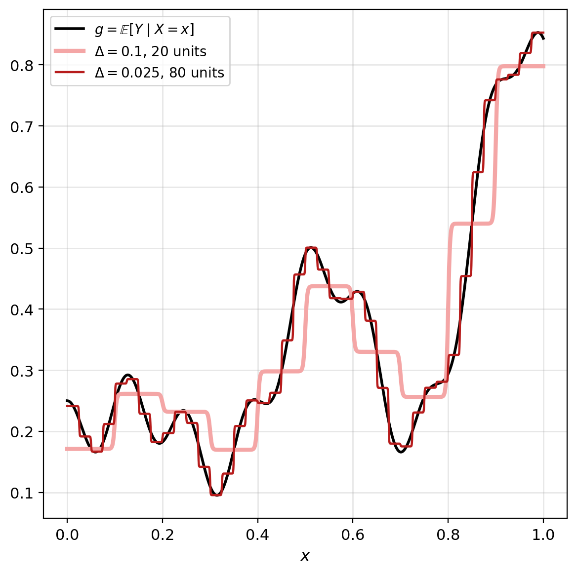
Example, every weight set from \(g\) (figure)
| \(\Delta\) | 0.2 | 0.1 | 0.05 | 0.025 | 0.0125 |
|---|---|---|---|---|---|
| hidden units | 10 | 20 | 40 | 80 | 160 |
| \(\max_x |h_\Delta - g|\) | 0.42 | 0.22 | 0.13 | 0.069 | 0.035 |
- Error about proportional to \(\Delta\): \(g\) has a bounded slope
The theorem for \(d = 1\): \(g\) continuous, so a small enough \(\Delta\) keeps \(g\) within \(\varepsilon\) of its value at each center, and a large enough \(w\) makes each bump a box
Networks Need Order \(\varepsilon^{-\mathrm{dim}/s}\) Units for Error \(\varepsilon\)
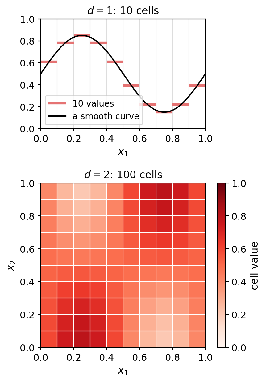
Cells in \(d\) dimensions: \(\Delta^{-d}\), one value each (figure)
- At \(\Delta = 0.1\): \(10\), \(100\), \(1{,}000\) for \(d = 1, 2, 3\)
- A \(28 \times 28\) image: \(10^{784}\)
Error proportional to \(\Delta\): half the error needs \(2^d\) times the cells, \(1{,}024\) times at \(d = 10\)
Networks, \(g\) with \(s\) bounded derivatives (DeVore, Howard, Micchelli 1989; Mhaskar 1996; Yarotsky 2017)
- Order \(\varepsilon^{-d/s}\) units for error \(\varepsilon\)
- \(s = 1\): the cell count above, with \(\Delta \propto \varepsilon\)
- The same order with one hidden layer or many
- No method with parameters continuous in \(g\) needs fewer
Trained Networks Miss Detail the Construction Represents
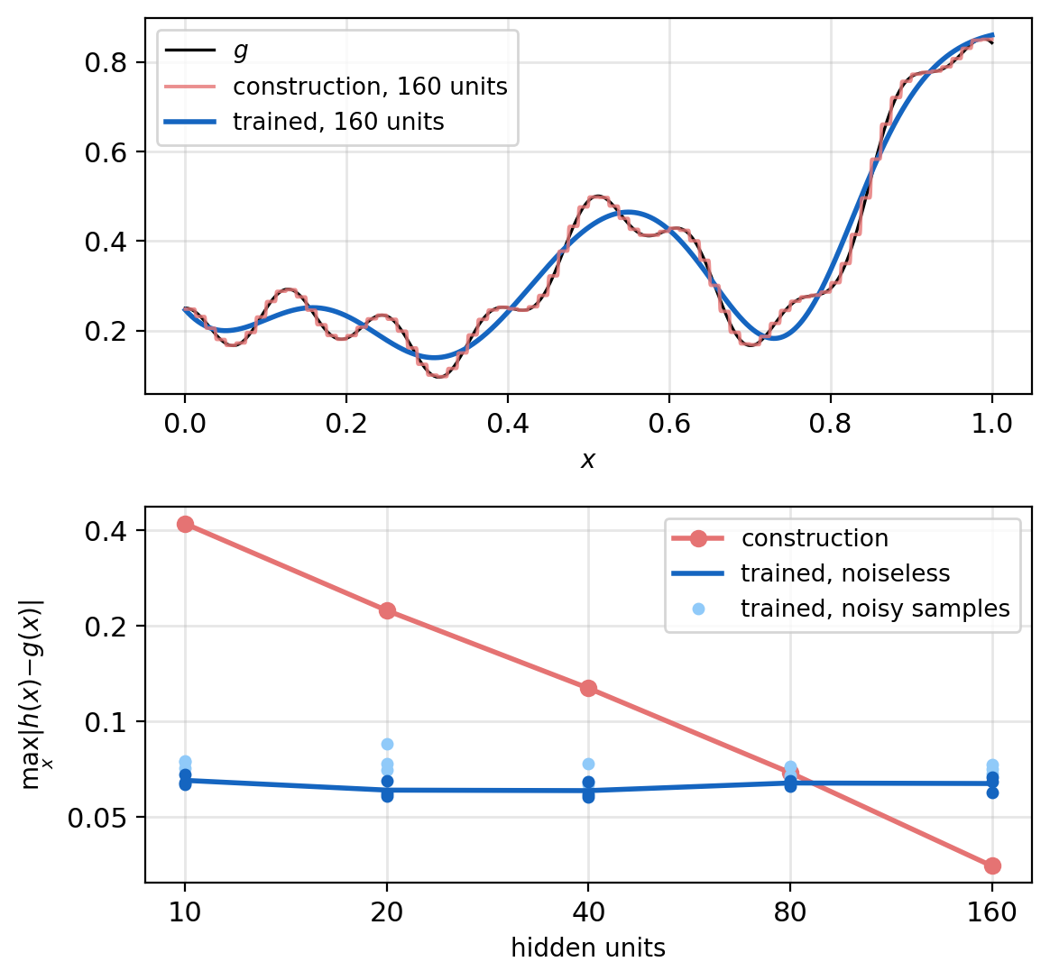
Training: one hidden layer of sigmoid units, full-batch Adam, \(20{,}000\) steps, three seeds, on \(1{,}000\) noiseless points of \(g\) itself
Maximum error \(\max_x |h(x) - g(x)|\)
| hidden units | 10 | 20 | 40 | 80 | 160 |
|---|---|---|---|---|---|
| construction | 0.42 | 0.22 | 0.13 | 0.069 | 0.035 |
| trained, noiseless | 0.065 | 0.061 | 0.061 | 0.064 | 0.064 |
- Below the construction at \(10\) to \(40\) units, above it at \(160\)
- Trained on the \(200\) noisy samples instead: \(0.06\) to \(0.09\)
Trained fits are smooth (figure): they miss the fast oscillation, at \(10\) units and at \(160\)
A ReLU Network Is a Different Linear Function in Each Region
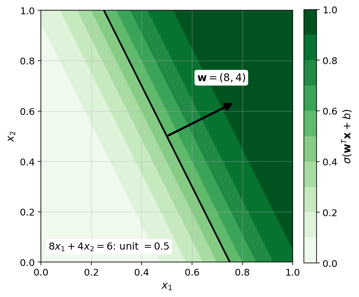
Hidden unit \(j\): \(\mathrm{ReLU}(\mathbf{w}_j^T \mathbf{x} + b_j)\)
- Equal to \(\mathbf{w}_j^T \mathbf{x} + b_j\) on one side of the line \(\mathbf{w}_j^T \mathbf{x} + b_j = 0\)
- Zero on the other side
Fixed on/off pattern: the network is the sum of its on units, a linear function of \(\mathbf{x}\)
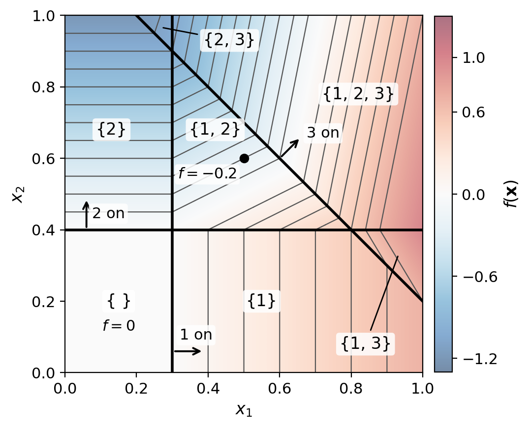
Example, three units on two inputs (figure): \(\mathbf{w}_1 = (1, 0)\), \(\mathbf{w}_2 = (0, 1)\), \(\mathbf{w}_3 = (1, 1)\), \(\mathbf{b} = (-0.3, -0.4, -1.2)\), \(\mathbf{v} = (1, -2, 1.5)\)
- Three lines cut the unit square into seven regions, one pattern each
- At \(\mathbf{x} = (0.5, 0.6)\), units \(1\) and \(2\) are on: \(f(\mathbf{x}) = (x_1 - 0.3) - 2(x_2 - 0.4) = -0.2\)
- Contours of \(f\): parallel within a region, a new direction across each line
Trained Weights Take the Shape of the Class a Unit Responds To
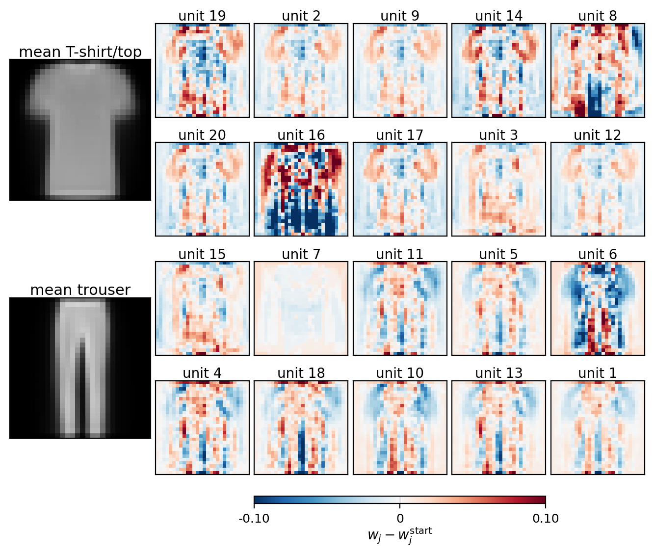
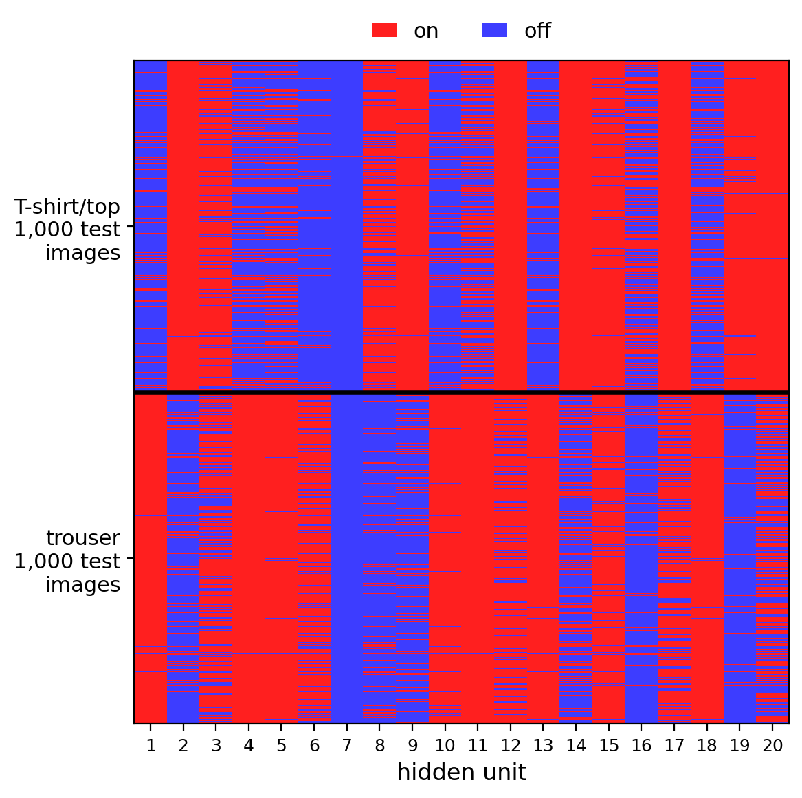
Network: one hidden layer of \(20\) ReLU units, FashionMNIST T-shirts/tops against trousers, \(99.05\%\) test accuracy
Weight change \(\mathbf{w}_j - \mathbf{w}_j^{\text{start}}\) of each unit, one value per pixel (figure)
- Red where a weight rose, blue where it fell, one scale for all \(20\) units
- Ordered from the most T-shirt-selective unit to the most trouser-selective
T-shirt units: weights rose over the shoulders, sleeves, and body
Trouser units: weights rose along the legs and fell in the gap between them
Match: \(\mathbf{w}_j^T \mathbf{x}\) is large when bright pixels meet positive weights
- Unit \(1\)’s weight change against the mean standardized image: \(4.18\) for trousers, \(-1.42\) for T-shirts
Second-Layer Units Can Respond to a Single Bounded Region
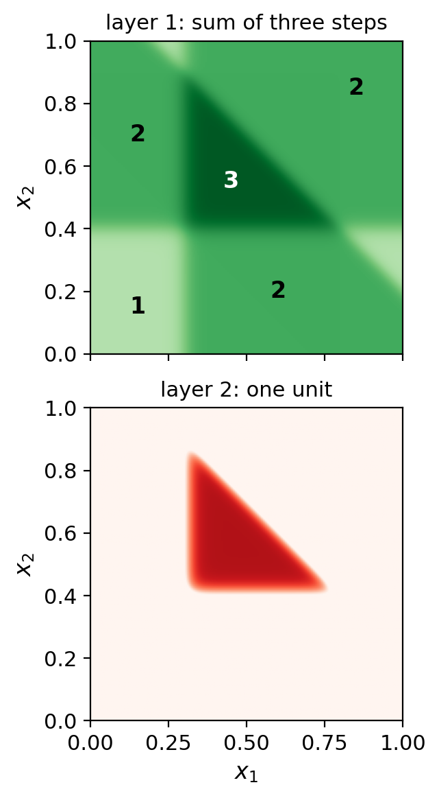
Layer 1: three steep steps, each near \(1\) on one side of a line
- \(x_1 > 0.3\), \(\;x_2 > 0.4\), \(\;x_1 + x_2 < 1.2\)
- Their sum: \(3\) inside the triangle, \(2\) or \(1\) elsewhere (figure, top)
Layer 2: one unit, \(2\,\mathrm{ReLU}(h_1 + h_2 + h_3 - 2.5)\)
- Positive only where all three steps are on (figure, bottom)
- \(0.99\) at \((0.4, 0.5)\), inside the triangle
- \(0\) at \((0.9, 0.9)\), \((0.1, 0.1)\), and \((0.5, 0.3)\)
One hidden layer: a sum of steps, each constant along its whole line, so no single unit is confined to a bounded region
Too-Deep Networks Do Not Train
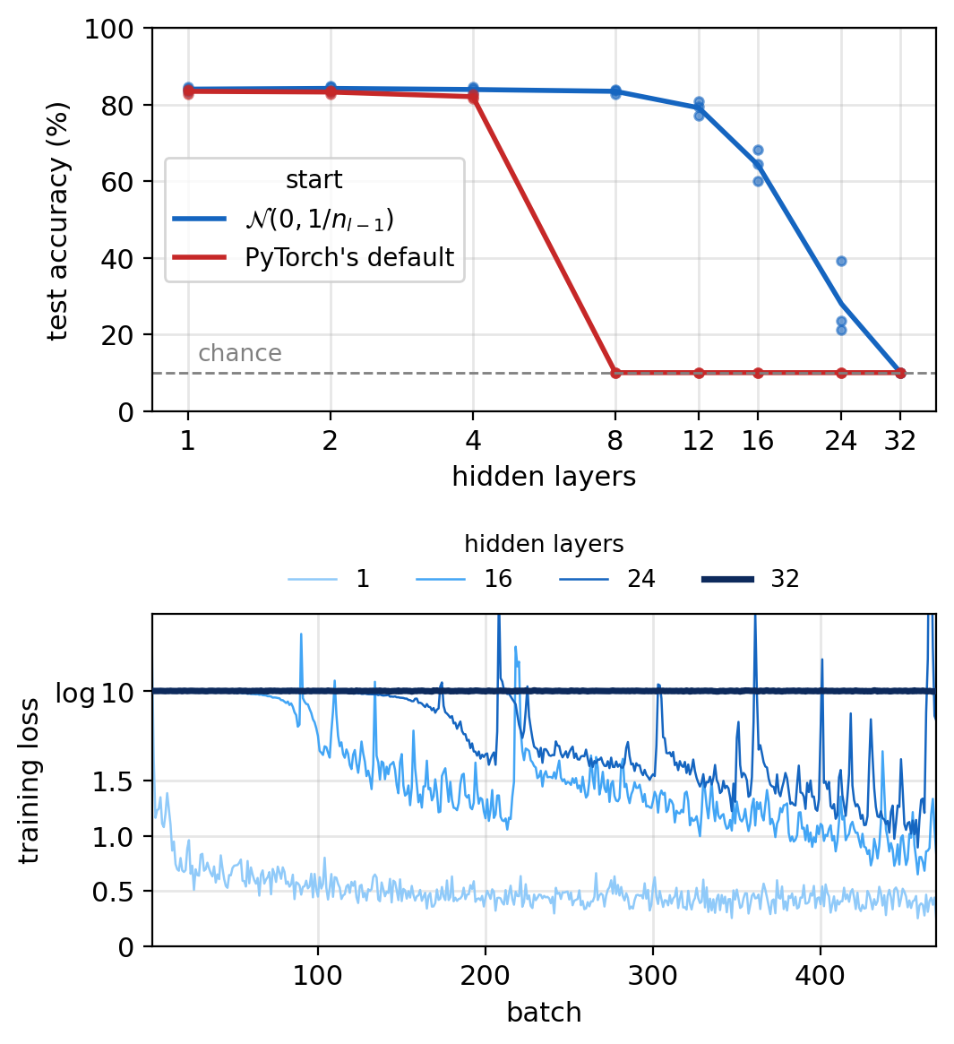
Networks: \(1\) to \(32\) hidden ReLU layers of \(256\) units, FashionMNIST
Training
- One epoch of SGD, \(\eta = 0.1\), batch \(128\)
- Three seeds per network
Starting weights, two choices
- \(\mathcal{N}(0, 1/n_{l-1})\), biases zero (lecture 06’s)
- PyTorch’s default
Test accuracy (top)
- \(\mathcal{N}(0, 1/n_{l-1})\): \(83\) to \(85\%\) up to \(8\) hidden layers, \(60\) to \(68\%\) at \(16\), chance (\(10\%\)) at \(32\)
- PyTorch’s default: chance from \(8\) hidden layers
Training loss (bottom), \(\mathcal{N}(0, 1/n_{l-1})\): at \(32\) hidden layers, \(\log 10 = 2.30\) on all \(469\) batches, the loss of a uniform guess over \(10\) classes
The Gradient Shrinks Exponentially With Depth
Backward pass, in row form, with \(\mathbf{D}^{(k)} = \mathrm{diag}\big(\sigma'(\mathbf{s}^{(k)})\big)\):
\[\boldsymbol{\delta}^{(l)T} = \boldsymbol{\delta}^{(L)T}\, \mathbf{W}^{(L)} \mathbf{D}^{(L-1)} \cdots \mathbf{W}^{(l+1)} \mathbf{D}^{(l)}\]
- One weight matrix and one slope matrix for every layer above \(l\)
- The first layer has the longest product
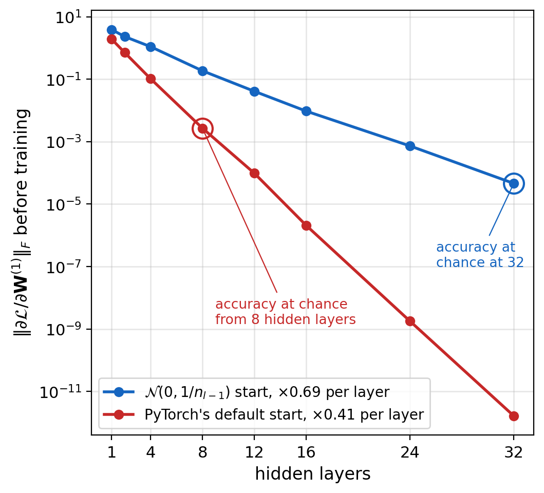
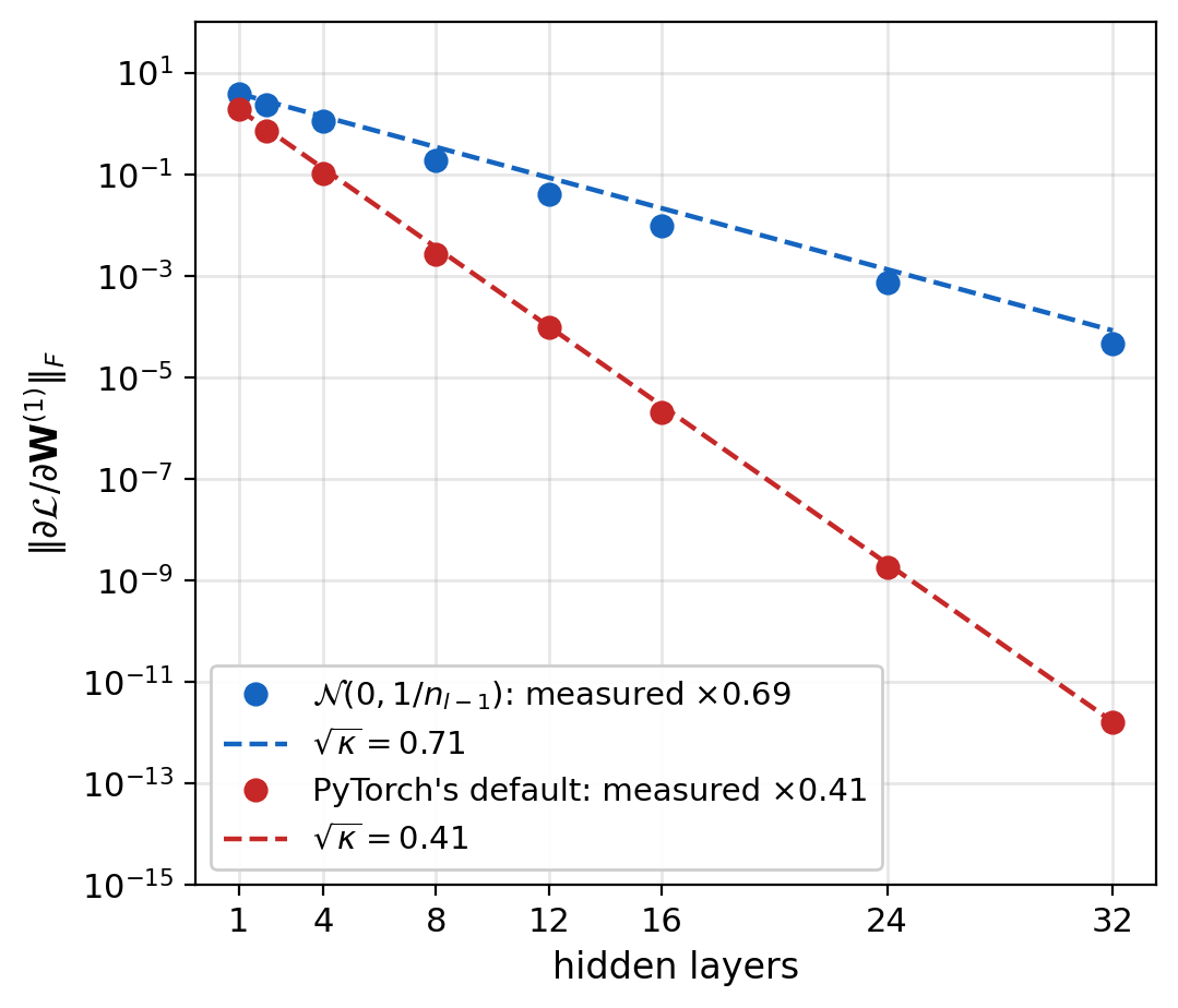
Measured: \(\|\partial \mathcal{L} / \partial \mathbf{W}^{(1)}\|_F\) before training, the networks of the depth sweep (figure)
- \(\mathcal{N}(0, 1/n_{l-1})\): \(\times 0.69\) per layer, from \(3.9\) at \(1\) hidden layer to \(4.6 \times 10^{-5}\) at \(32\)
- PyTorch’s default: \(\times 0.41\) per layer, from \(1.9\) to \(1.6 \times 10^{-12}\)
Backward pass exact at every depth: the gradient itself is small
Each Network Needs Its Own Hand-Derived Backward Pass
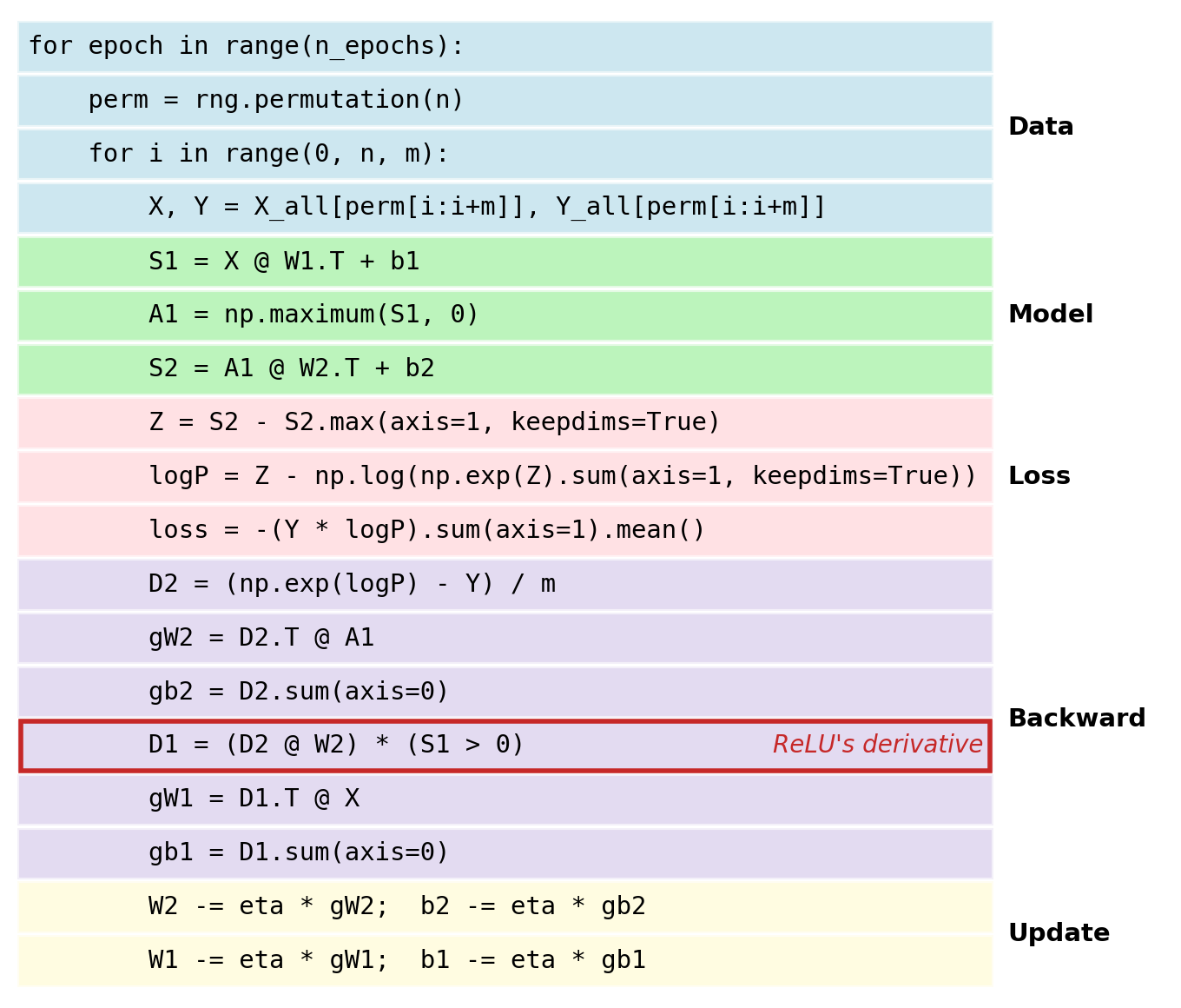
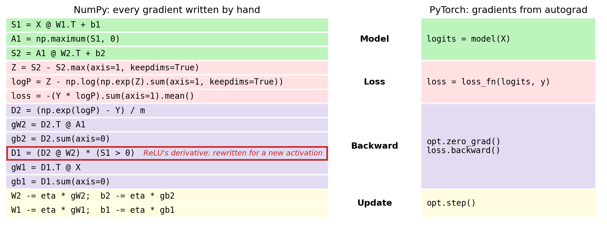
The NumPy training program, five blocks
- Data: a permutation of the indices, one slice per batch
- Model: the forward lines
- Loss: log-softmax and the mean
- Backward: six lines derived for this network; \((\mathbf{S}_1 > 0)\) in the line for
D1is ReLU’s derivative - Update: one gradient step per array
Changing the network: a new activation, layer, or loss changes the forward lines, and the backward lines must be derived again
PyTorch Computes the Backward Pass From the Recorded Forward Pass
PyTorch: an open-source Python library for building and training neural networks, first released by Facebook AI Research in 2016
- Tensors: arrays on a CPU or a GPU
- Autograd: operations on tensors recorded as they run, and
loss.backward()computes every gradient from that record torch.nn: layers that hold parameterstorch.optim: update rulestorch.utils.data: loading data in batches
Models Combine Modules That Hold Weights
Tensor: an array, such as a batch, a weight matrix, or a loss
Operation: a function of tensors, such as X @ W.T, torch.relu, F.cross_entropy
- Recorded as it runs when a tensor requires gradients
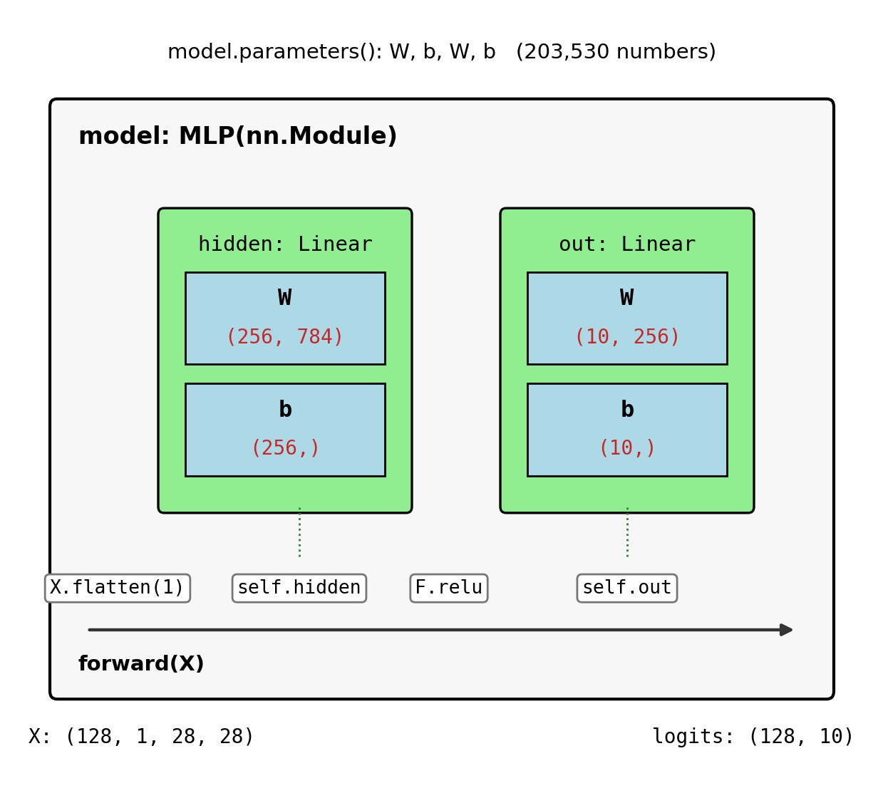
Module: an operation packaged with the tensors it keeps between calls, its parameters
nn.Linear(784, 256)holds \(\mathbf{W}\) and \(\mathbf{b}\)nn.ReLU()holds none
Model: a module whose forward applies modules and operations in any order Python allows (figure)
Optimizer: holds the model’s parameters and updates them
DataLoader: produces the batch tensors
Calling a Model Runs forward Between Its Hooks
Special methods: Python turns syntax into method calls
a + brunstype(a).__add__(a, b)model(X)runstype(model).__call__(model, X)
Hook: a function attached to a module that runs every time the module runs, for example to record its output
nn.Module.__call__, in order (figure)
- Forward pre-hooks, on the input
self.forward(X), the computation the class defines- Forward hooks, on the output
model.forward(X) called directly: steps 1 and 3 are skipped
class Double(nn.Module):
    def forward(self, x):
        return 2 * x

d = Double()
print(d(torch.tensor([1.0, 2.0])))
tensor([2., 4.])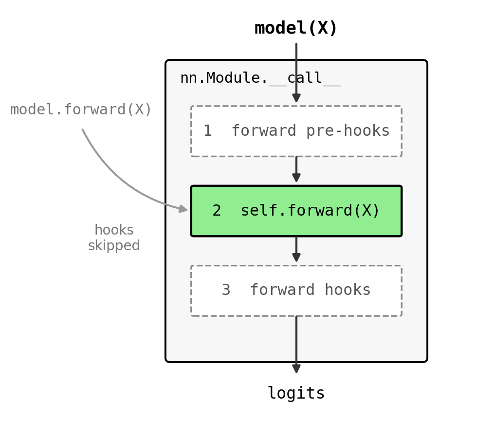
The Registry Holds Every Layer the Optimizer Updates
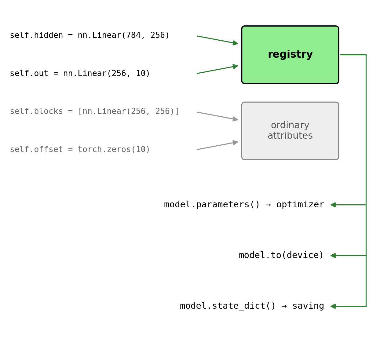
Assignment is a method call: self.name = value runs nn.Module.__setattr__
- A module or an
nn.Parametergoes into the model’s registry - Anything else, such as a plain tensor or a Python list, becomes an ordinary attribute
The registry feeds (figure)
model.parameters(), which the optimizer is givenmodel.to(device)model.state_dict(), which saving uses
Layers kept in a Python list: outside the registry
- The optimizer never updates them; they keep their random start
- The parameter count shows it: \(0\) for a list of two
Linearlayers, \(203{,}530\) withnn.ModuleList
Model and Batch Must Be on the Same Device
Devices
- CPU memory: always available
- GPU memory: CUDA on NVIDIA GPUs, MPS on Apple silicon (
float32only) - No local GPU: a hosted notebook with a GPU, such as Colab
Moves (figure)
model.to(device): every registered parameter, onceX.to(device): each batch, as it arrives- An operation on tensors from two devices is an error
Install and check
pip install torch torchvision
python -c "import torch; print(torch.cuda.is_available(), torch.backends.mps.is_available())"
if torch.cuda.is_available():
device = 'cuda'
elif torch.backends.mps.is_available():
device = 'mps'
else:
device = 'cpu'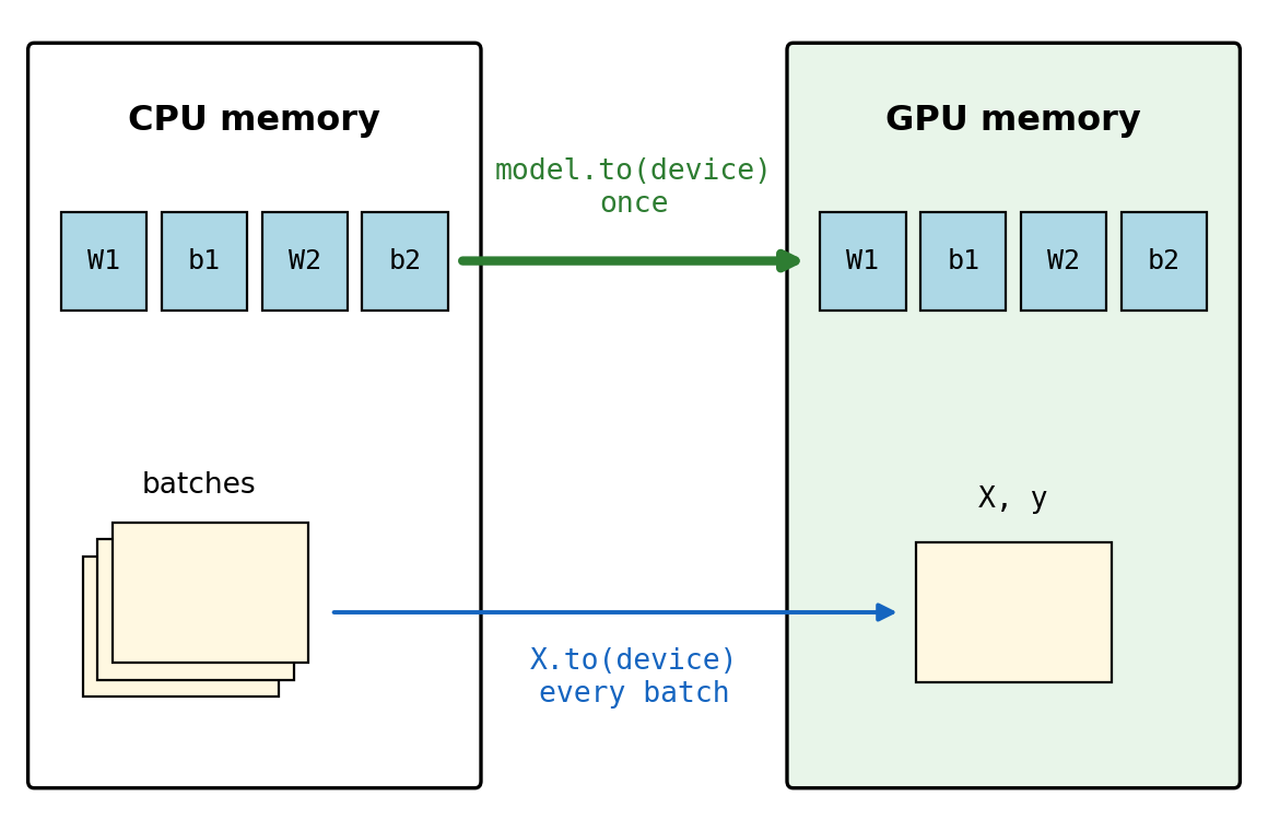
Tensors Work Like NumPy Arrays and Track Gradients Through Operations
Same as NumPy
- Shape, dtype,
@, broadcasting, slicing dim=where NumPy hasaxis=
Added (figure)
device: the memory holding the valuesrequires_grad: operations on the tensor are recordedgrad: filled bybackward(), the tensor’s shapegrad_fn: the recorded operation that produced it
Catches
float32by default, whiletorch.from_numpykeeps NumPy’sfloat64; afloat64batch into afloat32layer is an errortorch.from_numpy(a)andt.numpy()share memory with the other object.item()returns a plain number from a one-element tensor
w = torch.tensor([1.0, 2.0, 3.0], requires_grad=True)
f = (w ** 2).sum()
f.backward()
print(w.grad, f.grad_fn)
tensor([2., 4., 6.]) <SumBackward0 object at 0x701c3b74f0>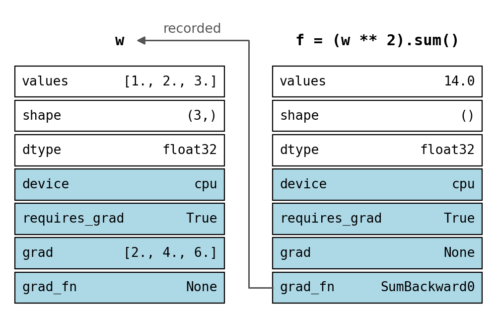
Flattened Image Batches Keep One Image per Row
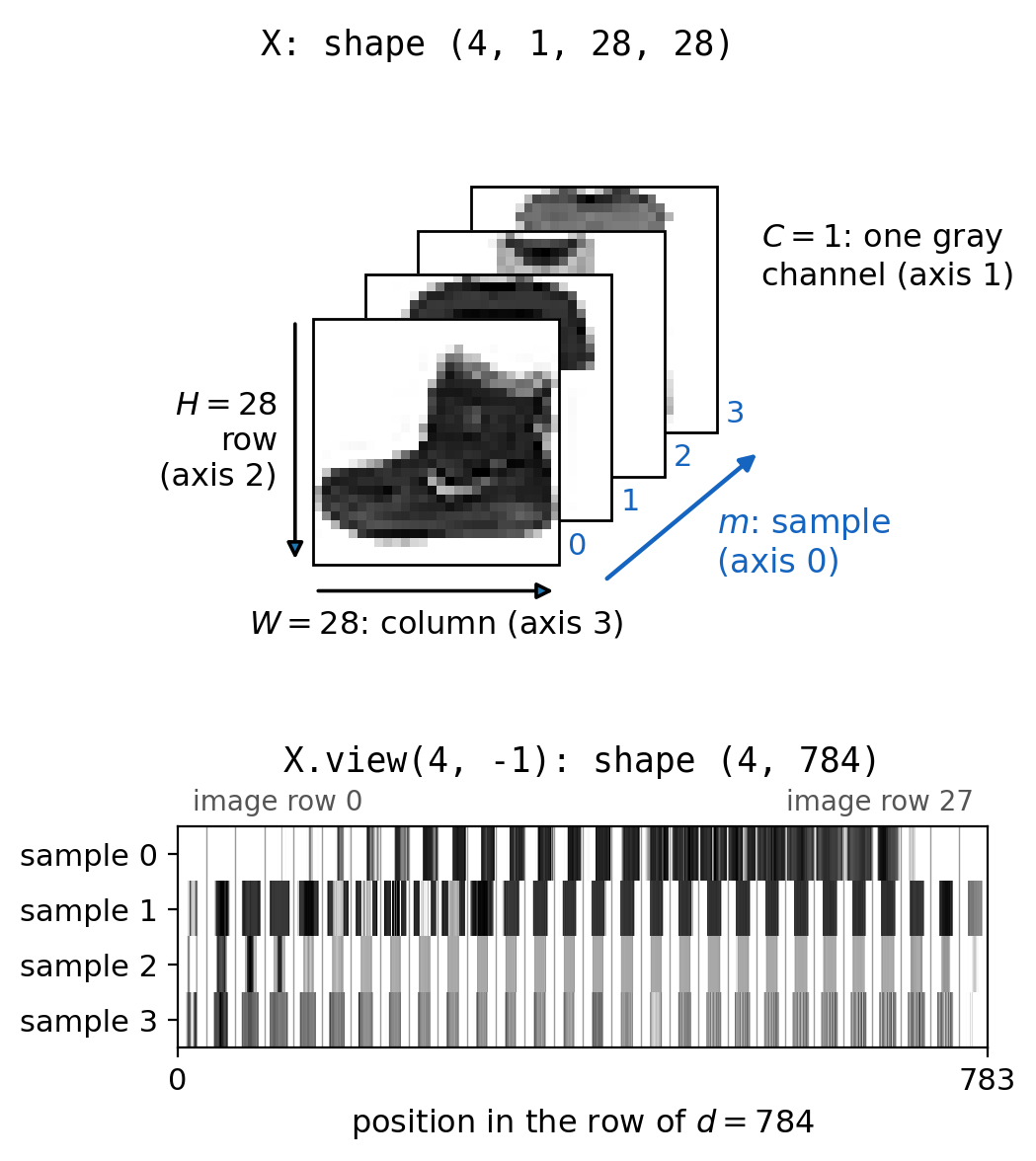
print(Xb.shape)             # (m, C, H, W)
print(Xb.flatten(1).shape)  # (m, d), d = C*H*W
torch.Size([128, 1, 28, 28])
torch.Size([128, 784])- \(m = 128\) images, \(C = 1\) gray channel (\(3\) for color), \(H = W = 28\) pixels
Xb.flatten(1)ornn.Flatten(): a new shape, the same memory
Flattened: one row of \(d = 784\) pixels per image, the \(m \times d\) input matrix \(\mathbf{X}\) of mini-batch backpropagation
With samples on the first axis, one matrix product computes a layer for the whole batch
Layers Allocate Their Weights When Created, So They Need Their Sizes
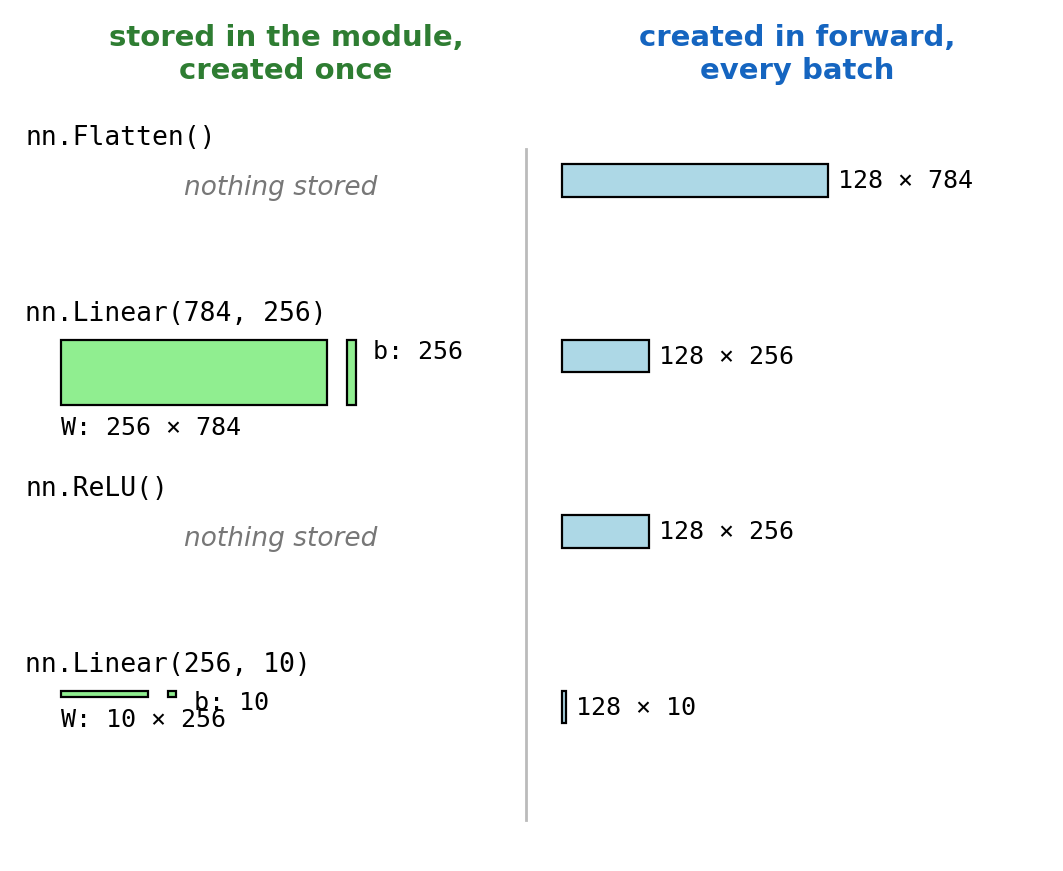
Created once, with the module (figure, left)
nn.Linear(784, 256): \(\mathbf{W}\) of \(256 \times 784\) and \(\mathbf{b}\) of \(256\), sized by the two argumentsnn.ReLU(),nn.Flatten(): nothing stored, so no sizes- Normalization layers store one value per feature, so they take the width as an argument too
Created at every forward pass (figure, right)
- Activations, one row per image: their size follows the batch
- Freed after
backward()uses them
A size mismatch: an error at the first forward pass, naming the two shapes
Most Training Programs Follow the Same Template
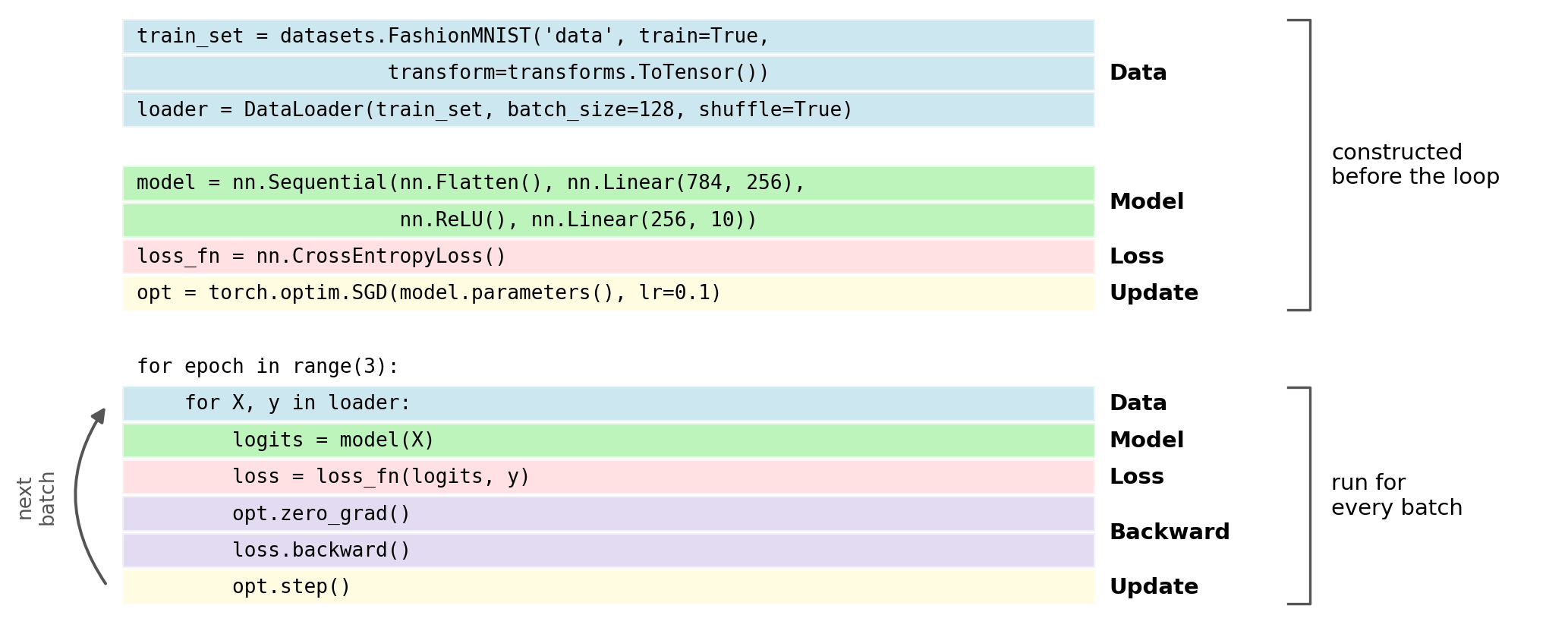
- Before the loop: each block’s objects are created once
- In the loop: Data Model Loss Backward Update, once per batch
- Run as written for \(3\) epochs: \(84.0\%\) test accuracy, about \(0.9\) s per epoch on the CPU
DataLoaders Feed the Dataset to the Model

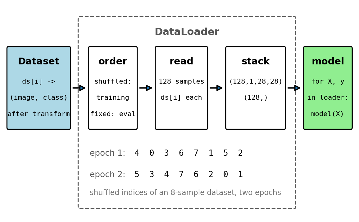
Dataset: one sample at a time
train_set[i]: an image, \((1, 28, 28)\), and its classlen(train_set): \(60{,}000\)- Transforms run as each sample is read:
ToTensor()here, resizing, normalizing, or random crops elsewhere
DataLoader: delivers samples to the model in batches
- Order: shuffled each epoch for training, fixed for validation and test
- Read: the next \(128\) samples, in parallel worker processes if requested
- Stack: \((128, 1, 28, 28)\) and \((128,)\)
Shuffling: different samples share a gradient step each epoch
One epoch: \(469\) batches of \(128\), so \(469\) gradient steps
loader = DataLoader(train_set, batch_size=128, shuffle=True)
for X, y in loader:      # iter(loader), then next() per batch
    ...
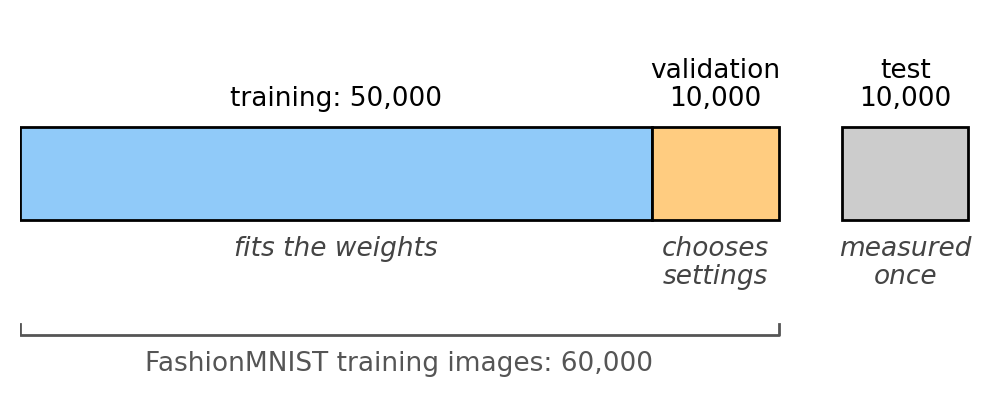
Test Data Is Held Back Until Every Choice Is Made
Training set: gradient descent fits the weights to it
Validation set: compares the settings gradient descent does not fit
- Learning rate, number of epochs, architecture, penalty \(\lambda\)
Test set: used once, after every choice
- Any choice made by looking at it biases its error low
FashionMNIST has \(60{,}000\) training and \(10{,}000\) test images
- The validation set comes from the training images
Size: an accuracy near \(88\%\) measured on \(n\) images has standard error \(\sqrt{0.88 \cdot 0.12 / n}\)
- \(0.3\) percentage points at \(n = 10{,}000\)
- \(1.0\) at \(n = 1{,}000\)
full = datasets.FashionMNIST('data', train=True,
            transform=transforms.ToTensor())
train_set, val_set = random_split(
    full, [50_000, 10_000],
    generator=torch.Generator().manual_seed(0))

loader = DataLoader(train_set, batch_size=128,
                    shuffle=True)
val_loader = DataLoader(val_set, batch_size=1000)
print(len(train_set), len(val_set), len(loader))
50000 10000 391CrossEntropyLoss Applies the Softmax, So Models Output Logits

Logits: the model’s raw class scores, any real numbers
nn.CrossEntropyLoss(): log-softmax and negative log-likelihood in one function
- \(\ell = \log \sum_k e^{s_k} - s_y\), computed as log-sum-exp so large scores do not overflow
- Inputs: logits \((m, K)\) and class indices \((m,)\)
A softmax in the model too: the loss then applies a second softmax, to probabilities
- \(\ell = 0.702\) instead of \(0.241\) in the example
- With \(K = 10\) classes, \(\ell \geq 1.46\) for any output
Two classes: one output with nn.BCEWithLogitsLoss(), equivalent to two outputs with one score fixed at \(0\)
Regression: nn.MSELoss() broadcasts outputs \((m, 1)\) against targets \((m,)\) to \((m, m)\), with only a warning
logits = torch.tensor([[2.0, 0.5, -1.0]])
y1 = torch.tensor([0])
loss_fn = nn.CrossEntropyLoss()

print(loss_fn(logits, y1))
print(loss_fn(logits.softmax(1), y1))      # wrong
tensor(0.2413)
tensor(0.7017)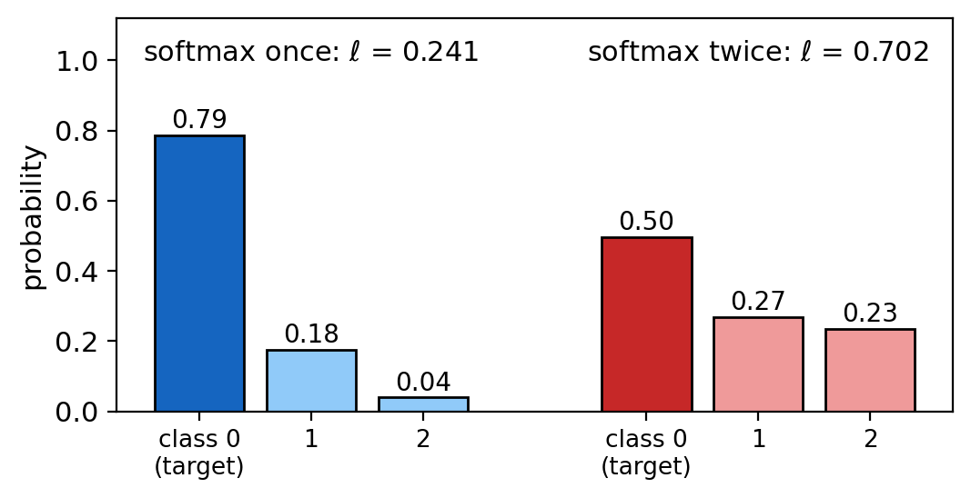
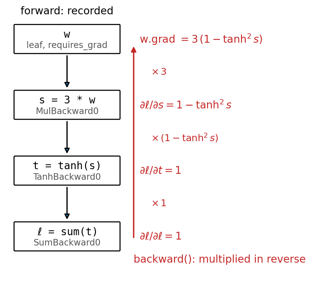
backward() Computes Every Gradient From a Recorded Forward Pass

Forward pass: each operation on a tensor that requires gradients is recorded, with what its local derivative needs
backward(): the chain rule over the record, from the loss back to each parameter
- Each gradient lands in its parameter’s
.grad - Then the record is freed, and the next forward pass makes a new one
Checked: a tanh, ReLU, and sigmoid network whose gradients were never derived by hand
- \(102\) gradients against finite differences, largest difference below \(10^{-8}\)
Gradients Accumulate. zero_grad() Clears Them.
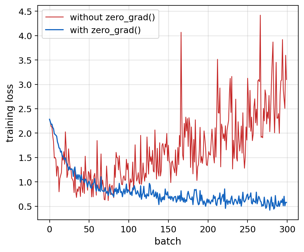
backward() adds to the existing .grad
w = torch.tensor(2.0, requires_grad=True)
(w ** 2).backward()
(w ** 2).backward()
print(w.grad) # 2w + 2w, not 2wtensor(8.)Without opt.zero_grad(): each step uses the sum of all gradients so far, and training fails
Accumulation on purpose: backward() on \(k\) small batches, each loss divided by \(k\), then one step
- The step uses the gradient of the mean loss over the \(k\) batches
- A large batch’s gradient with a small batch’s memory
opt.step() Applies the Update Rule to Every Parameter

The optimizer receives model.parameters() once and keeps a reference to each tensor
opt.step() for SGD, written out
with torch.no_grad():
    for p in model.parameters():
p -= 0.1 * p.grad- In place, so the optimizer’s references stay valid
- Inside
no_grad(), so the update is not recorded
A different update rule: a different optimizer class, and nothing else changes
opt = torch.optim.Adam(model.parameters(), lr=1e-3)torch.manual_seed(0)
lin = nn.Linear(3, 1)
opt = torch.optim.SGD(lin.parameters(), lr=0.1)
lin(torch.ones(1, 3)).sum().backward()
params = list(lin.parameters())
by_hand = [p - 0.1 * p.grad for p in params]
opt.step()
print([torch.allclose(p, q)
for p, q in zip(params, by_hand)])[True, True]Monitoring Training: The Validation Curve Shows Overfitting
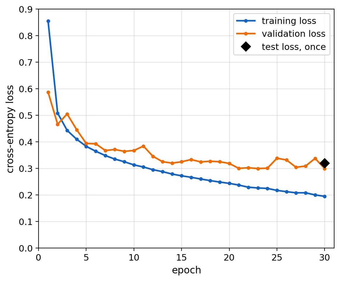
The template program, with a validation set
- \(50{,}000\) training and \(10{,}000\) validation images
- Two hidden layers of \(256\) ReLU units, SGD with \(\eta = 0.1\), batch \(128\), \(30\) epochs
Recorded every epoch
- Training loss:
loss.item()from each of the \(391\) batches, averaged - Validation loss: after the epoch, under
model.eval()andtorch.no_grad() - Logging
lossinstead ofloss.item()keeps every batch’s record in memory
Measured
- Training: \(0.85\) at epoch \(1\), \(0.20\) at epoch \(30\)
- Validation: between \(0.30\) and \(0.34\) from epoch \(14\) on
- The widening gap is overfitting: the model fits the training images better without fitting new images better
Test, once, at the end: loss \(0.32\), accuracy \(88.9\%\)
Frameworks Do Not Produce Bit-Identical Results
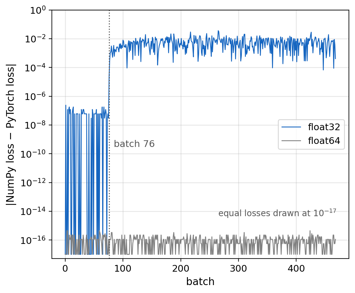
Same network, starting weights, and batch order: \(784\)-\(256\)-\(256\)-\(10\), ReLU, SGD with \(\eta = 0.1\), batch \(128\), one epoch
- NumPy: the hand-written lines
- PyTorch: the template loop, on the CPU and on the Apple GPU
Test accuracy
- NumPy: \(85.3\%\)
- PyTorch: \(85.3\%\) on the CPU, \(85.2\%\) on the Apple GPU
Loss per batch
- Within \(3 \times 10^{-7}\) for \(76\) batches
- Then apart by more than \(10^{-3}\) within three batches, at most \(0.04\)
In float64: within \(10^{-15}\) for the whole epoch, so the drift is float32 rounding, amplified by training
Reproducibility: the same program on two frameworks or two devices agrees to rounding at first, not bit for bit over a run
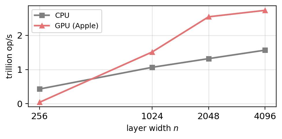
Large Layers Run Faster on the GPU, Small Layers on the CPU
A GPU: thousands of arithmetic units, and a fixed cost for every call (launching the work, waiting for the result)
Work per step, forward and weight gradient of a square ReLU layer: \(4mn^2\) operations
- \(n = 256\), \(m = 128\): \(34\) million
- \(n = 4096\), \(m = 2048\): \(137\) billion
Operations per second achieved
- \(n = 256\): CPU \(0.43\) trillion, GPU \(0.04\) trillion
- \(n = 4096\): CPU \(1.6\) trillion, GPU \(2.7\) trillion
Small layers: too little work to cover the GPU’s fixed cost
Time per step
- \(n = 256\): CPU \(0.08\) ms, GPU \(0.80\) ms
- \(n = 4096\): CPU \(88\) ms, GPU \(50\) ms
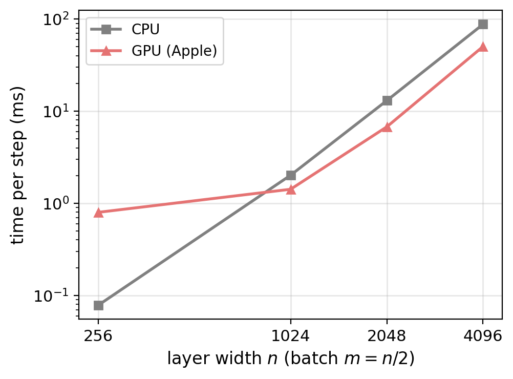
Copying: the training set to the Apple GPU and back takes 20 ms, against 0.9 s for one CPU epoch
Hooks Inject Code Into the Forward and Backward Pass
Forward hook: a function called with a layer’s output each time the layer runs
Tensor hook: a function called with a tensor’s gradient during backward()
Uses: recording outputs or gradients, extracting features, changing a gradient before it is used (a hook that returns a value replaces the gradient)
Example: recording the size of every hidden layer’s output and gradient
torch.manual_seed(0)
layers = [nn.Linear(784, 256), nn.ReLU()]
for _ in range(5):
    layers += [nn.Linear(256, 256), nn.ReLU()]
deep = nn.Sequential(*layers, nn.Linear(256, 10))
fwd, bwd = [], []

def record(layer, inputs, out):
    fwd.append(out.std().item())
    out.register_hook(
        lambda g: bwd.insert(0, g.std().item()))

for layer in deep[:-1]:
    if isinstance(layer, nn.Linear):
        layer.register_forward_hook(record)

X_h = torch.randn(512, 784)
y_h = torch.randint(0, 10, (512,))
F.cross_entropy(deep(X_h), y_h).backward()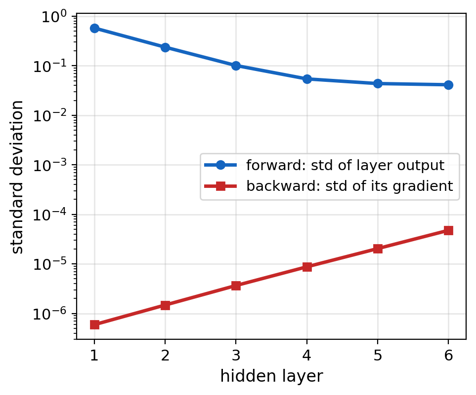
- One forward and one backward pass: the output and gradient size of every hidden layer
At Initialization, Signal Size Changes by a Fixed Gain per Layer
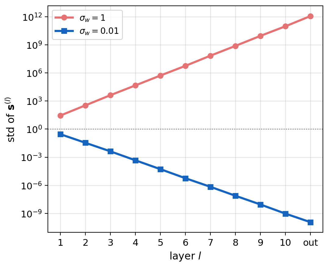
Network: \(10\) hidden layers of \(256\) ReLU units, \(10\) outputs, biases zero
- Weights from \(\mathcal{N}(0, \sigma_w^2)\) with \(\sigma_w = 1\) and \(\sigma_w = 0.01\)
- \(512\) FashionMNIST images, standardized, \(\mathbb{E}[x^2] = 1.02\)
Measured with forward hooks, before any training: the spread of each layer’s pre-activations \(\mathbf{s}^{(l)}\)
s_std = []
def record(layer, inputs, out):
    s_std.append(out.std().item())

for m in net:
    if isinstance(m, nn.Linear):
        m.register_forward_hook(record)
net(X)          # one forward pass fills s_std
Factor per layer, hidden layers \(2\) to \(10\)
- \(\sigma_w = 1\): \(\times 10.6\) to \(\times 12.2\)
- \(\sigma_w = 0.01\): \(\times 0.106\) to \(\times 0.122\)
Output: \(1.2 \times 10^{12}\) and \(1.2 \times 10^{-10}\), from a factor of \(100\) in \(\sigma_w\)
Training Fails When the Signal Explodes or Vanishes
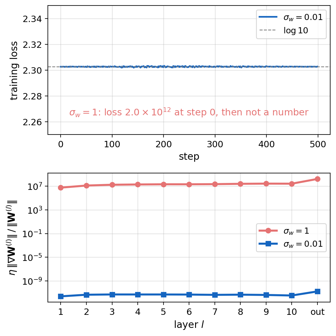
Training: SGD, \(\eta = 0.01\), batch \(128\), \(500\) steps
\(\sigma_w = 1\)
- First loss \(2.0 \times 10^{12}\)
- One step moves each weight matrix by \(5 \times 10^{6}\) to \(2 \times 10^{8}\) times its own norm
- The next forward pass overflows to \(\pm\infty\), and every later loss is NaN
\(\sigma_w = 0.01\)
- Loss \(2.303 = \log 10\) for all \(500\) steps, the uniform guess over \(10\) classes
- One step moves each weight matrix by \(3 \times 10^{-12}\) to \(2 \times 10^{-11}\) of its norm
Relative step \(\eta\, \|\nabla \mathbf{W}^{(l)}\| / \|\mathbf{W}^{(l)}\|\): the same order of magnitude at every layer, so the overall scale is wrong, not particular layers
Independent Products: \(\mathrm{Var}(wx) = \mathbb{E}[w^2]\,\mathbb{E}[x^2]\)
Conditions: \(w\) and \(x\) independent, \(\mathbb{E}[w] = 0\)
\[\mathrm{Var}(wx) = \mathbb{E}[w^2 x^2] - \big(\mathbb{E}[w]\,\mathbb{E}[x]\big)^2 = \mathbb{E}[w^2]\,\mathbb{E}[x^2]\]
- \(\mathbb{E}[x^2]\), not \(\mathrm{Var}(x)\): the mean of \(x\) counts
- \(\mathbb{E}[wx] = 0\) whatever the mean of \(x\)
A sum of \(n\) such products, the weights independent of each other and of the \(x_i\)
\[\mathrm{Var}\Big(\sum_{i=1}^{n} w_i x_i\Big) = n\, \mathbb{E}[w^2]\, \mathbb{E}[x^2]\]
- The terms are uncorrelated even when the \(x_i\) are correlated, so their variances add
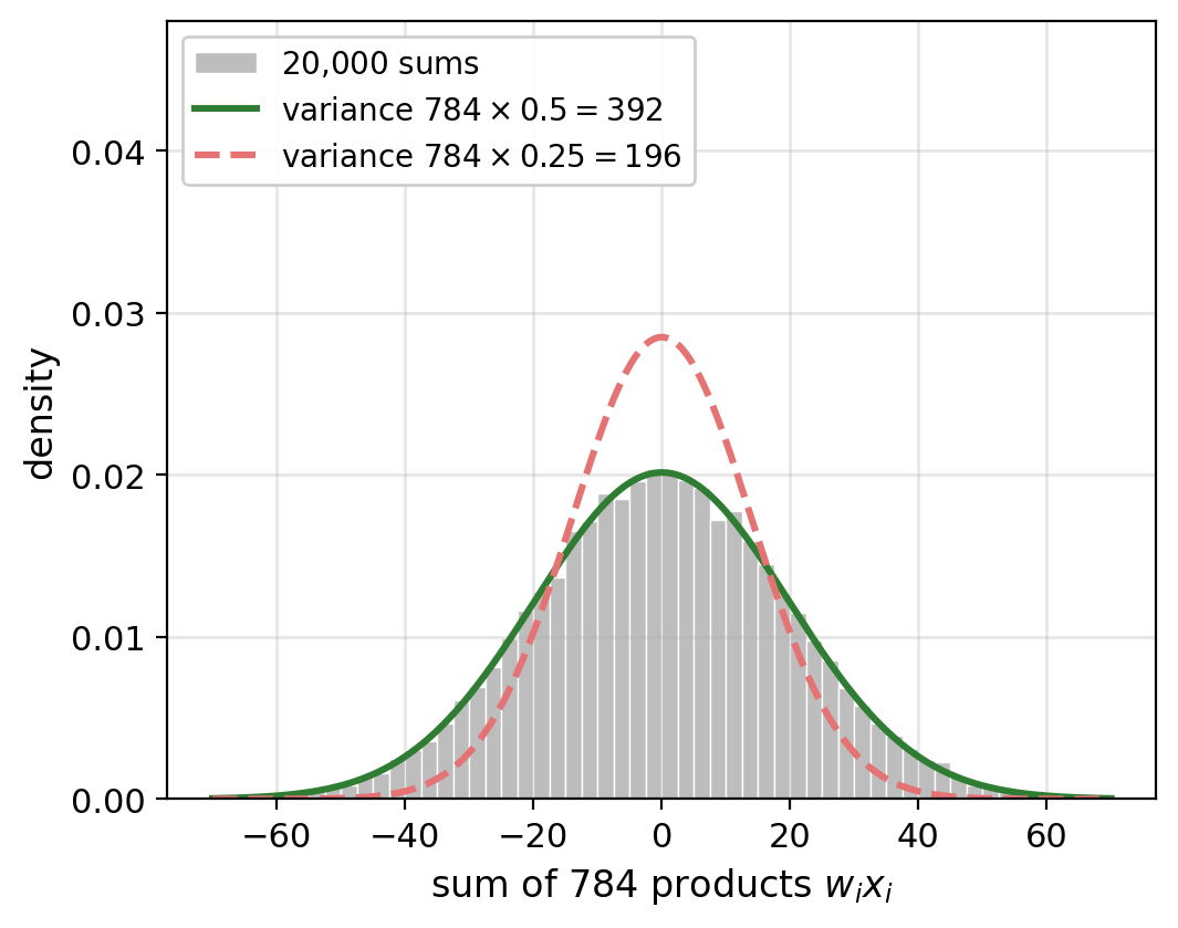
Example: \(w \sim \mathcal{N}(0, 0.5^2)\), \(x \sim \mathcal{N}(1, 1)\)
- \(\mathrm{Var}(wx) = 0.25 \times 2 = 0.5\), not \(0.25 \times 1\)
- A sum of \(784\) terms: \(392\)
A pre-activation \(s_i = \sum_j w_{ij} a_j\) is such a sum
ReLU Keeps Half the Second Moment of a Symmetric Signal
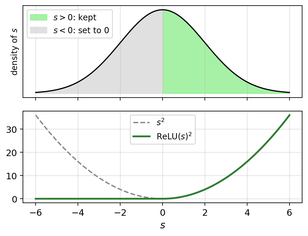
Symmetric \(s\): \(s\) and \(-s\) have the same distribution, as a zero-mean Gaussian does
ReLU sets the negative half to zero and keeps the positive half unchanged
\[\mathbb{E}\big[\mathrm{ReLU}(s)^2\big] = \mathbb{E}\big[s^2\, \mathbf{1}\{s > 0\}\big] = \tfrac{1}{2}\, \mathbb{E}[s^2]\]
- By symmetry, the positive half carries half of \(\mathbb{E}[s^2]\)
- \(\mathbb{E}[s^2] = \mathrm{Var}(s)\) when \(\mathbb{E}[s] = 0\)
ReLU’s slope: \(1\) for \(s > 0\), \(0\) otherwise
\[\mathbb{E}\big[\mathrm{ReLU}'(s)^2\big] = P(s > 0) = \tfrac{1}{2}\]
Example: \(s \sim \mathcal{N}(0, 4)\)
- \(\mathbb{E}[s^2] = 4.00\), \(\mathbb{E}[\mathrm{ReLU}(s)^2] = 2.00\), \(P(s > 0) = 0.50\), from \(10^6\) draws
- Any symmetric distribution gives the same half
Forward Pass: Each Layer Multiplies \(\mathrm{Var}(s)\) by \(\kappa = n_{l-1}\, \sigma_w^2 / 2\)
Pre-activation of unit \(i\) in layer \(l\)
\[s_i^{(l)} = \sum_{j=1}^{n_{l-1}} w_{ij}^{(l)}\, a_j^{(l-1)}, \qquad \mathrm{Var}\big(s^{(l)}\big) = n_{l-1}\, \sigma_w^2\, \mathbb{E}\big[(a^{(l-1)})^2\big]\]
- At the random start the weights are independent of \(\mathbf{a}^{(l-1)}\), which depends only on earlier layers
ReLU: \(\mathbb{E}\big[(a^{(l-1)})^2\big] = \tfrac{1}{2} \mathrm{Var}\big(s^{(l-1)}\big)\), so
\[\mathrm{Var}\big(s^{(l)}\big) = \kappa\, \mathrm{Var}\big(s^{(l-1)}\big), \qquad \kappa = \frac{n_{l-1}\, \sigma_w^2}{2}\]
The example, \(n_{l-1} = 256\)
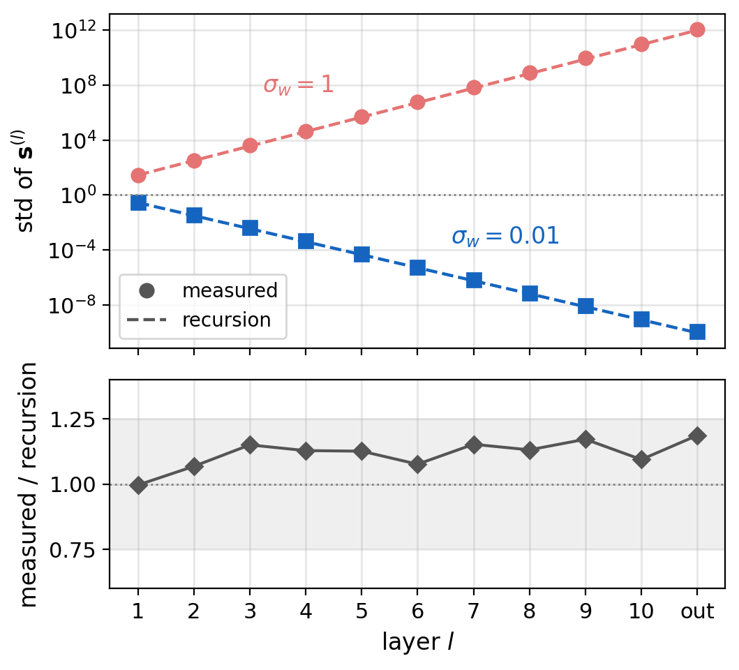
- \(\sigma_w = 1\): \(\kappa = 128\), standard deviation \(\times 11.3\) per layer
- \(\sigma_w = 0.01\): \(\kappa = 0.0128\), \(\times 0.113\)
- Layer 1: \(784\, \sigma_w^2\, \mathbb{E}[x^2]\), standard deviation \(28.3\) at \(\sigma_w = 1\)
Measured: within \(25\%\) of the recursion at every hidden layer
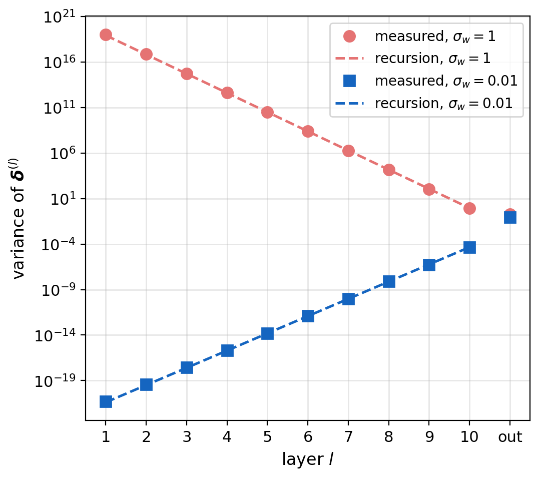
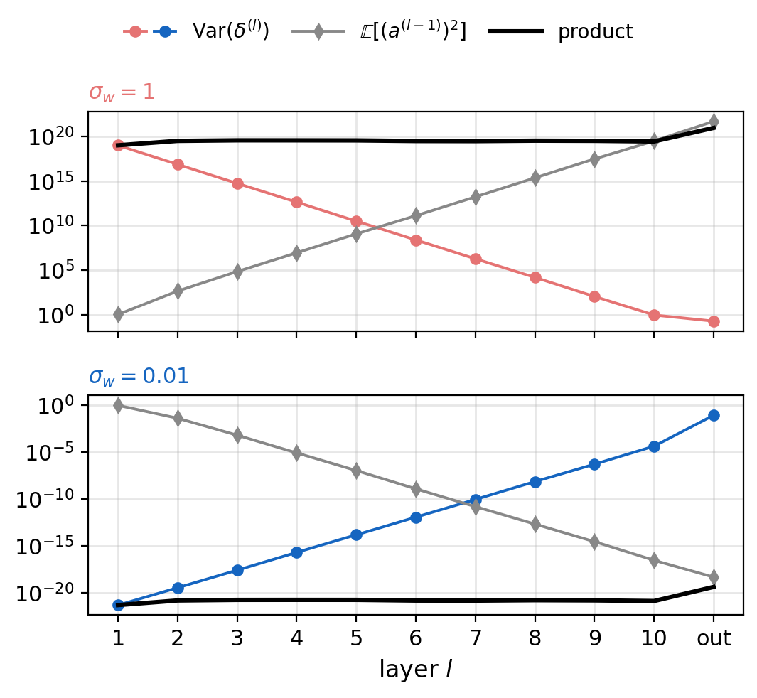
Backward Pass: Each Layer Multiplies \(\mathrm{Var}(\delta)\) by the Same \(\kappa\)
Backward recursion, from the output toward the input
\[\boldsymbol{\delta}^{(l)} = \big(\mathbf{W}^{(l+1)T} \boldsymbol{\delta}^{(l+1)}\big) \odot \sigma'\big(\mathbf{s}^{(l)}\big)\]
- Each entry of \(\mathbf{W}^{(l+1)T} \boldsymbol{\delta}^{(l+1)}\): a sum of \(n_{l+1}\) products \(w\,\delta\)
- Then multiplied by ReLU’s slope, with \(\mathbb{E}[\sigma'^2] = \tfrac{1}{2}\)
Approximation: the weights treated as independent of \(\boldsymbol{\delta}^{(l+1)}\), checked against the measurement
\[\mathrm{Var}\big(\delta^{(l)}\big) = \frac{n_{l+1}\, \sigma_w^2}{2}\, \mathrm{Var}\big(\delta^{(l+1)}\big)\]
- Equal widths: the same \(\kappa\) as the forward pass, applied from the output down
Measured with tensor hooks: within \(10\%\) of \(128\) and \(0.0128\) per layer
\(\sqrt{\kappa}\) Predicts the Gradient Shrinkage Across Depth
Measured in the Depth section: the first layer’s gradient shrinks by a fixed factor per added layer
Predicted: each layer multiplies the gradient’s variance by \(\kappa\), so its norm by \(\sqrt{\kappa}\)
\(\mathcal{N}(0, 1/n_{l-1})\) weights: \(\sigma_w^2 = 1/n_{l-1}\)
- \(\kappa = \tfrac{1}{2}\), \(\sqrt{\kappa} = 0.71\)
- Measured: \(\times 0.69\) per layer
PyTorch’s default nn.Linear weights: uniform on \(\pm 1/\sqrt{n_{l-1}}\)
- \(\sigma_w^2 = 1/(3 n_{l-1})\), the variance of a uniform distribution
- \(\kappa = \tfrac{1}{6}\), \(\sqrt{\kappa} = 0.41\)
- Measured: \(\times 0.41\) per layer
Both starts: \(\kappa < 1\), so deep networks start with vanishing gradients
Small Gain Errors Compound Over Many Layers
Gain per layer, forward and backward
\[\kappa = \underbrace{n_{l-1}}_{\text{fan-in}} \times \underbrace{\sigma_w^2}_{\text{weight variance}} \times \underbrace{\tfrac{1}{2}}_{\text{ReLU}}\]
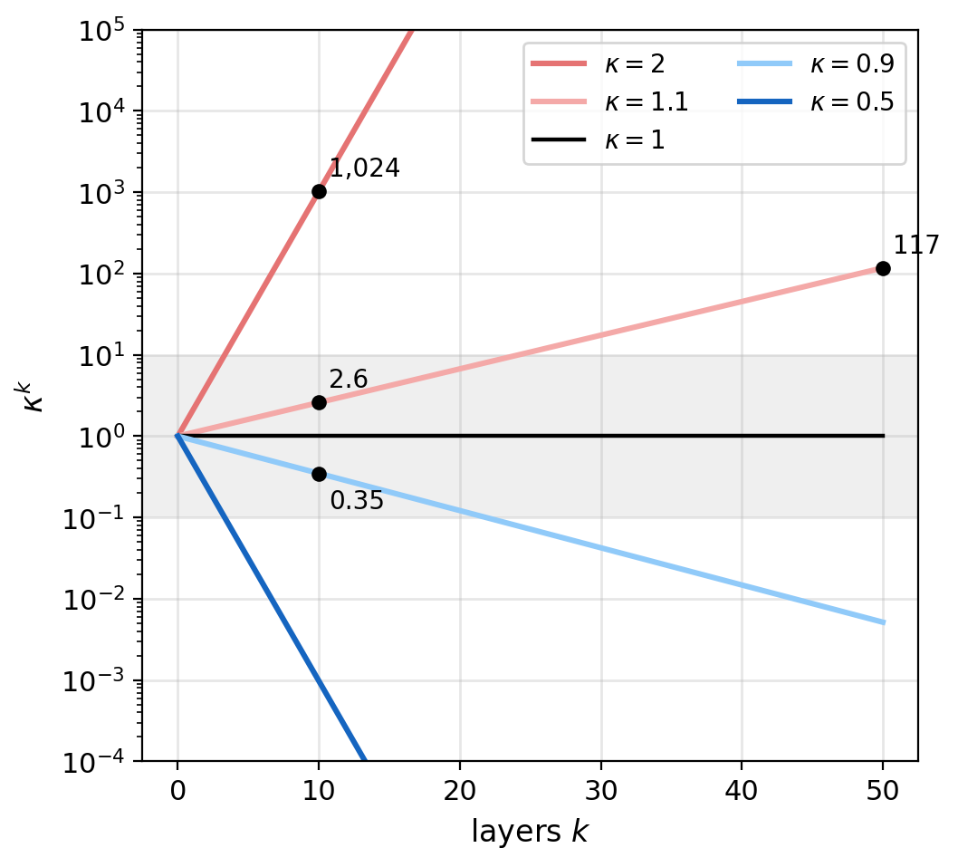
After \(k\) layers: the variance times \(\kappa^k\)
- \(k = 10\): \(\kappa = 1.1\) gives \(2.6\), \(\kappa = 0.9\) gives \(0.35\)
- \(k = 50\): \(\kappa = 1.1\) gives \(117\)
A deep network needs \(\kappa\) close to \(1\) at every layer, not only of order \(1\)
- The fan-in is fixed by the architecture
- The factor \(\tfrac{1}{2}\) comes from the activation
- The weight variance \(\sigma_w^2\) is set when the weights are drawn
The Activation Contributes a Factor to the Gain in Each Direction
Signal Propagation’s recursions with a general activation \(\sigma\), \(n\) units per layer
\[\mathrm{Var}\big(s^{(l)}\big) = n\, \sigma_w^2\; \mathbb{E}\big[\sigma(s^{(l-1)})^2\big]\]
\[\mathrm{Var}\big(\delta^{(l)}\big) = n\, \sigma_w^2\; \mathbb{E}\big[\sigma'(s^{(l)})^2\big]\, \mathrm{Var}\big(\delta^{(l+1)}\big)\]
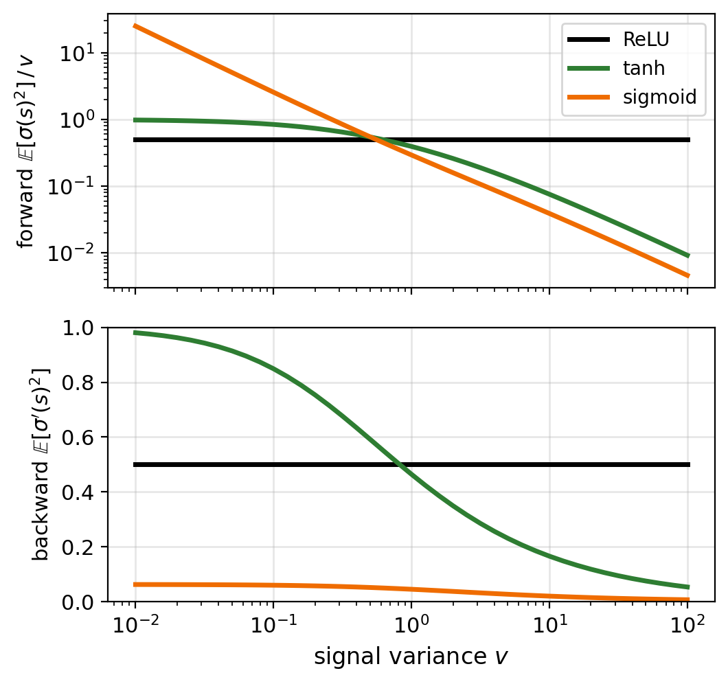
Activation factors, for \(s \sim \mathcal{N}(0, v)\)
- Forward: \(\mathbb{E}[\sigma(s)^2] / v\)
- Backward: \(\mathbb{E}[\sigma'(s)^2]\)
- \(s\) is close to Gaussian: a sum of \(n\) independent products
ReLU: both factors \(\tfrac{1}{2}\) at every \(v\)
- \(\mathrm{ReLU}(c\, s) = c\, \mathrm{ReLU}(s)\) for \(c > 0\), and the slope depends only on the sign of \(s\)
Tanh and sigmoid: each factor depends on \(v\), and the two factors differ
Sigmoid and Tanh Flatten for Large \(|s|\)
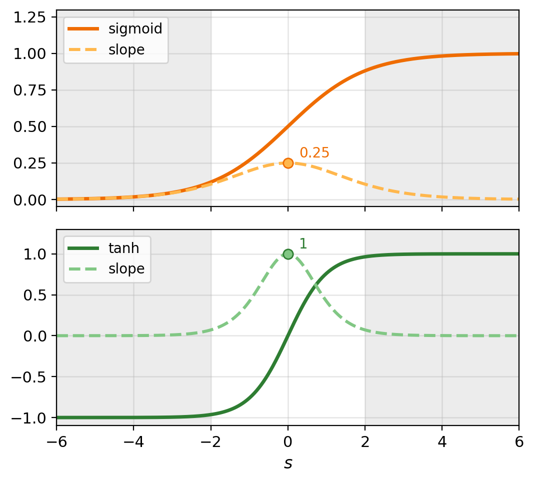
Sigmoid \(\dfrac{1}{1 + e^{-s}}\), slope \(\mathrm{sigmoid}(s)\big(1 - \mathrm{sigmoid}(s)\big)\)
- Largest slope \(\tfrac{1}{4}\), at \(s = 0\), so the backward factor is at most \(\tfrac{1}{16}\) at every \(v\)
- Output in \((0, 1)\), mean \(\tfrac{1}{2}\) for symmetric \(s\): \(\mathbb{E}[a^2] = \mathrm{Var}(a) + \tfrac{1}{4} \geq \tfrac{1}{4}\) at every \(v\)
Tanh \(= 2\, \mathrm{sigmoid}(2s) - 1\), slope \(1 - \tanh^2(s)\)
- Slope \(1\) at \(s = 0\): close to the identity for small \(s\)
- Slope below \(0.071\) wherever \(|s| > 2\) (sigmoid: below \(0.105\))
Saturation: the share of units with \(|s| > 2\), for \(s \sim \mathcal{N}(0, v)\)
- \(v = 0.1\): \(0.0\%\)
- \(v = 10\): \(53\%\), and tanh’s backward factor falls from \(0.85\) to \(0.17\)
Sigmoid Gradients Vanish While the Forward Variance Is Constant
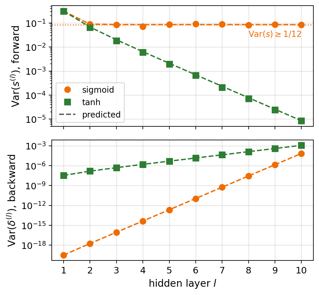
Network: Signal Propagation’s, \(10\) hidden layers of \(256\) units, biases zero, PyTorch’s default weights: \(\mathrm{Var}(w) = 1/(3n)\), so \(n\, \sigma_w^2 = \tfrac{1}{3}\)
Sigmoid
- Forward: \(\mathbb{E}[a^2] \geq \tfrac{1}{4}\), so \(\mathrm{Var}(s) \geq \tfrac{1}{3} \cdot \tfrac{1}{4} = 0.083\) in expectation: measured \(0.07\) to \(0.09\) from layer \(2\) on
- Backward: \(\tfrac{1}{3}\, \mathbb{E}[\sigma'(s)^2] = 0.020\) per layer, measured \(0.018\) to \(0.021\)
- Weight gradient: \(1.6 \times 10^{-8}\) in layer \(1\), \(0.46\) at the output
Tanh, close to the identity at small \(s\)
- Both factors near \(1\), so forward and backward \(\times \tfrac{1}{3}\) per layer: measured \(0.31\) to \(0.35\)
- Weight gradients of the same size at every layer, as with ReLU
Same-size weight gradients need the forward and backward factors to match
Saturated Tanh Bounds the Signal and Multiplies the Gradient
Weights from \(\mathcal{N}(0, 1)\): \(n\, \sigma_w^2 = 256\), same network with tanh
Forward: \(|a| \leq 1\), so \(\mathrm{Var}(s) \leq 256\)
- Measured: \(242\) to \(244\) from layer \(3\) on
- ReLU at this scale: \(\times 128\) per layer
- \(90\%\) of activations have \(|a| > 0.96\) at every layer from \(3\) on
Backward: \(256\, \mathbb{E}[\sigma'(s)^2]\) at \(v = 244\), predicted \(8.7\) per layer, measured \(8.3\) to \(9.1\)
- Weight gradient: \(6 \times 10^{4}\) in layer \(1\), \(1.2\) at the output
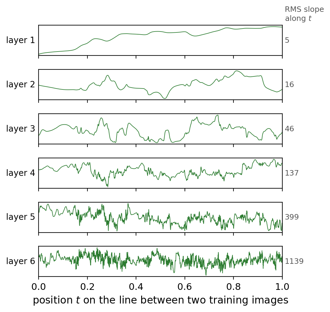
Repeated composition: inputs on the line between two training images, through layers \(1\) to \(6\)
- The slope along the line grows \(\times 2.9\) to \(\times 3.0\) per layer: \(\sqrt{8.7} = 2.9\)
- Each layer adds more and steeper oscillations, within a bounded range
ReLU’s Factor Is \(\tfrac{1}{2}\) for Every Variance of \(s\)
Scaling: for \(c > 0\)
\[\mathrm{ReLU}(c\, s) = c\, \mathrm{ReLU}(s), \qquad \mathrm{ReLU}'(c\, s) = \mathrm{ReLU}'(s)\]
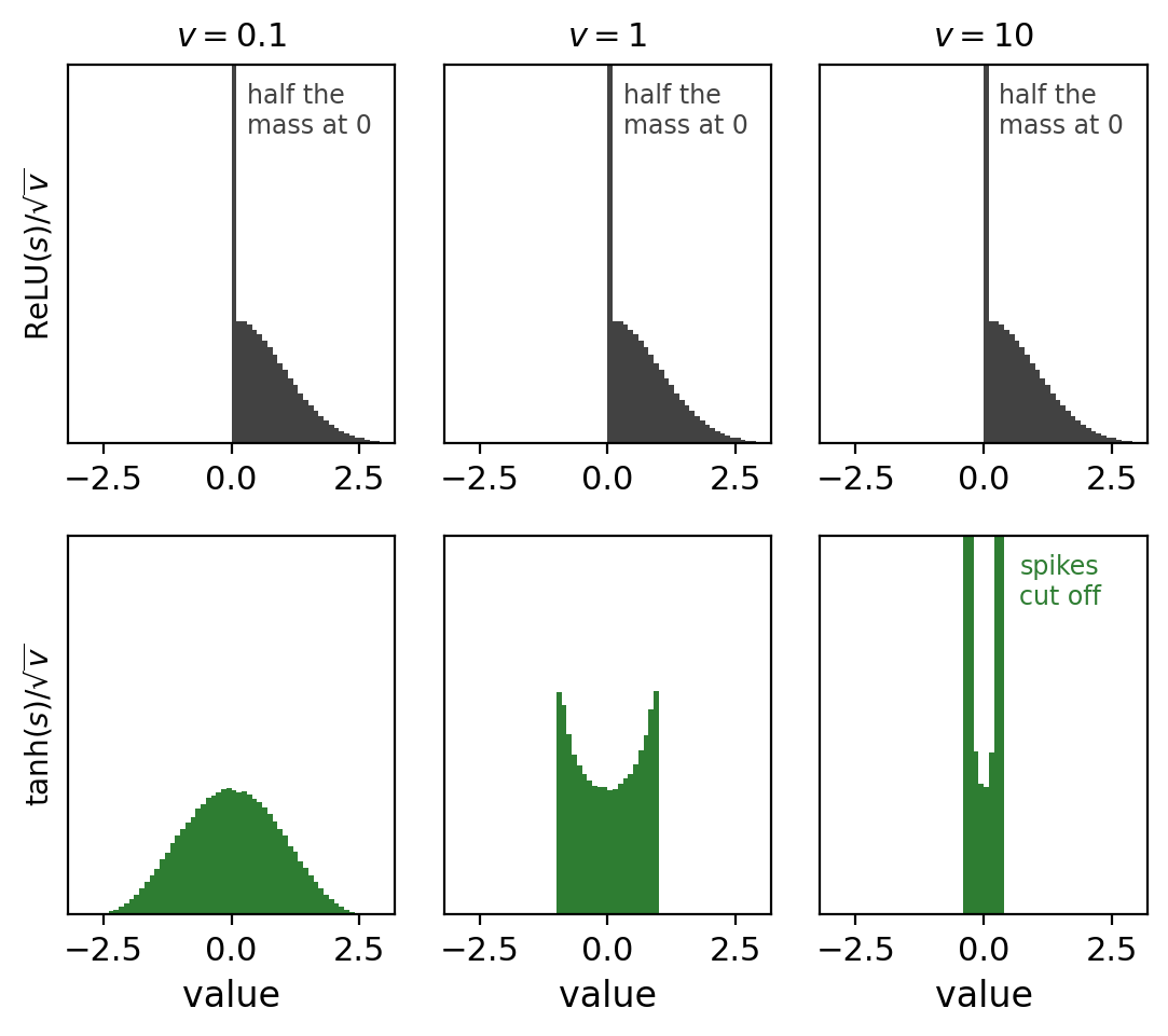
- Scaling \(s\) scales the output and leaves the slope, so the shape of \(\mathrm{ReLU}(s)/\sqrt{v}\) does not depend on \(v\)
- Tanh’s shape does: \(|a| > 0.96\) for \(0.0\%\) of units at \(v = 0.1\), \(54\%\) at \(v = 10\)
One gain, \(\kappa = n\, \sigma_w^2 / 2\), at every layer and in both directions
- The weight scale alone sets it: \(\sigma_w = 0.01\) still vanishes, and PyTorch’s default shrinks \(\times 0.41\) per layer
- ReLU does not remove vanishing gradients: it makes them fixable by the weight variance
At \(s = 0\) ReLU has no derivative, and PyTorch uses \(0\)
- A continuous \(s\) is exactly \(0\) with probability \(0\)
Dead ReLU Units Get No Gradient
Dead unit: \(s \leq 0\) on every training input, so its slope is \(0\) on every input
- Its incoming weights and its bias get zero gradient
- No gradient passes through it to earlier layers
- It turns back on only if changes in earlier layers move its inputs
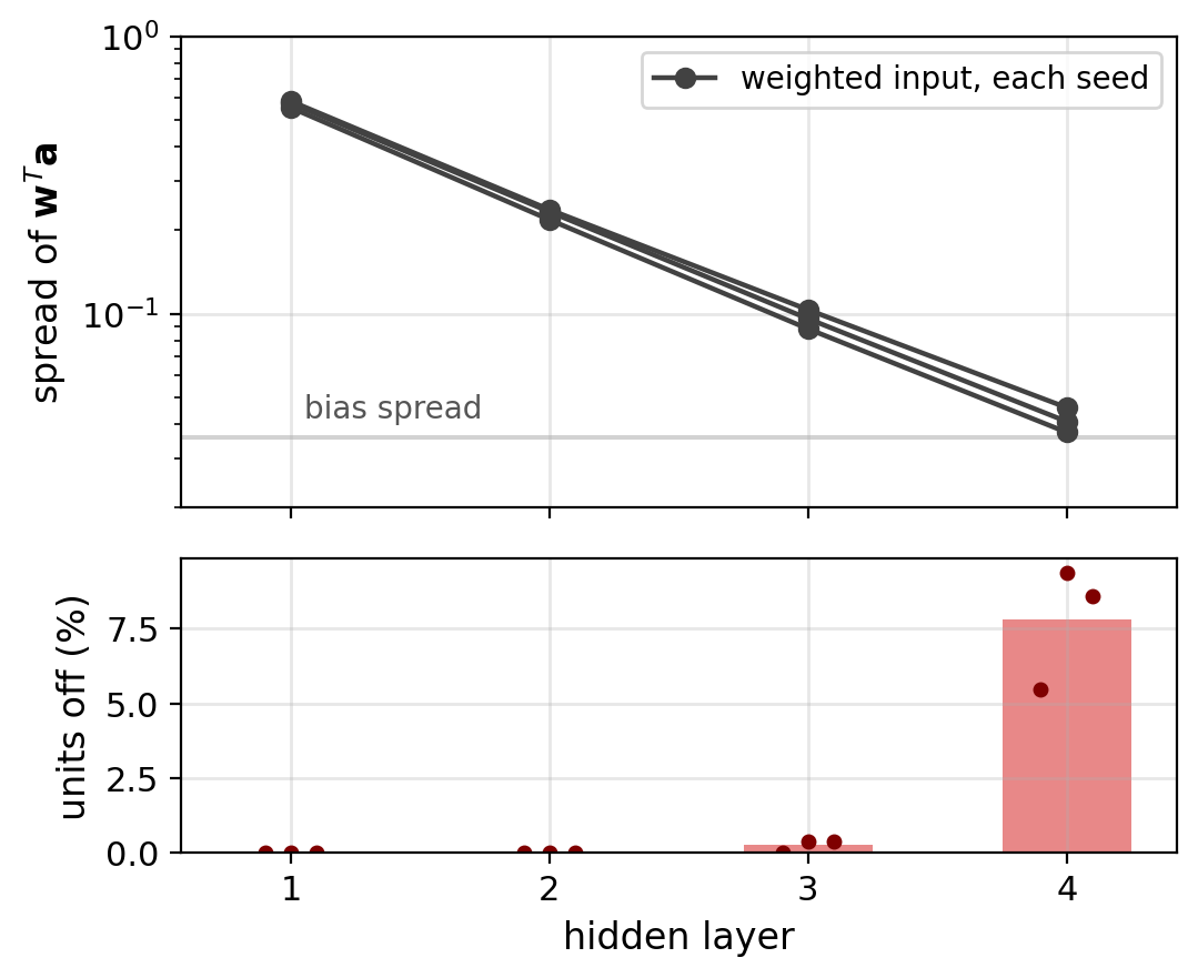
At PyTorch’s default start, with its default biases: \(4\) hidden layers of \(256\) units, \(3\) seeds
- Layer \(4\): \(5.5\%\) to \(9.4\%\) of units off before any step
- The weighted input \(\mathbf{w}^T \mathbf{a}\) shrinks \(\times 0.39\) to \(\times 0.44\) per layer, close to \(\sqrt{\kappa} = 0.41\): spread \(0.55\) to \(0.58\) in layer \(1\), \(0.04\) to \(0.05\) in layer \(4\)
- The biases’ spread is \(0.04\), so in layer \(4\) the bias decides the sign
- \(92\%\) to \(95\%\) of the units off at the start have a negative bias
Large Learning Rates Create Dead Units
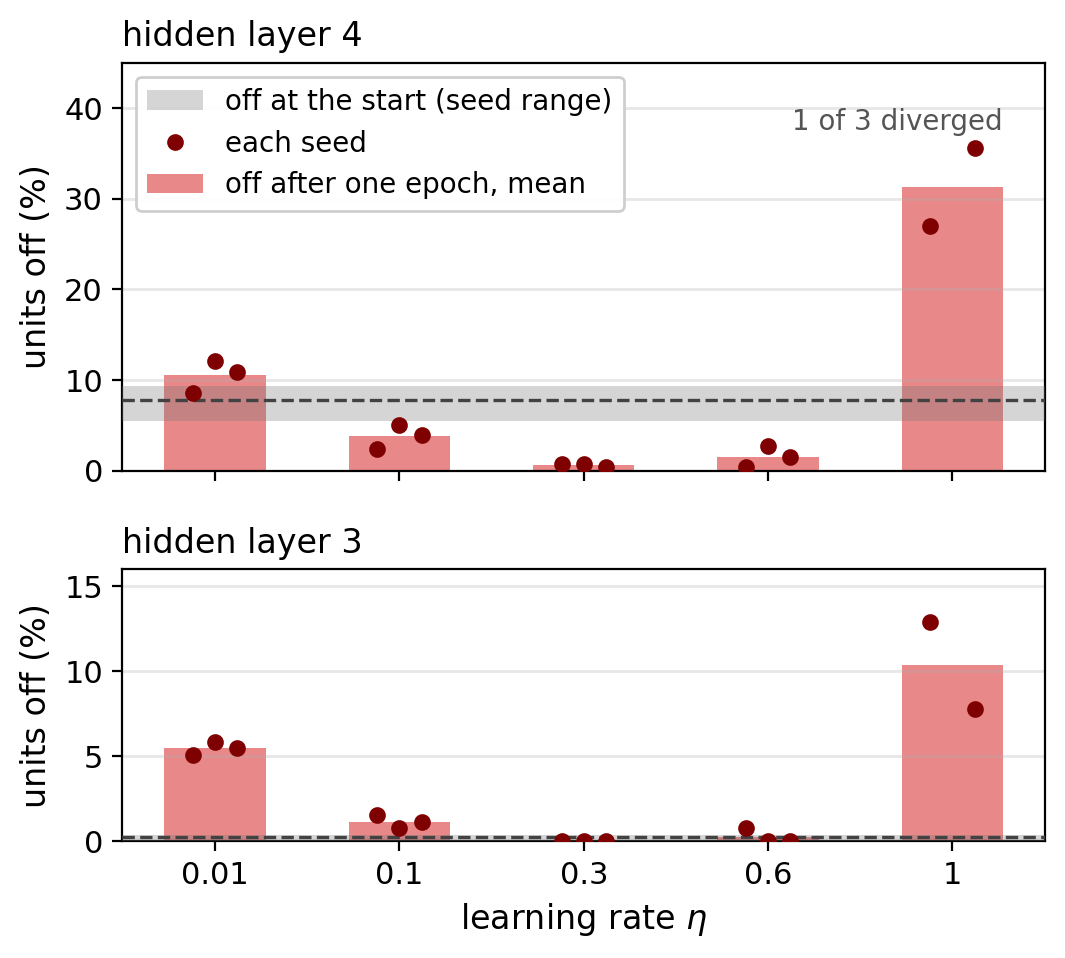
Units off in layer 4 after one epoch of SGD from the same start, batch \(128\), \(3\) seeds
- \(\eta = 0.01\): \(8.6\%\) to \(12.1\%\), above the start in every seed by \(2.3\) to \(3.1\) points
- \(\eta = 0.3\): \(0.4\%\) to \(0.8\%\), test accuracy \(83\)-\(84\%\)
- \(\eta = 1.0\): \(27\%\) and \(36\%\), test accuracy \(68\%\) and \(77\%\)
- \(\eta = 1.0\), third seed: the loss diverges
Mechanism
- One large update can move a unit’s bias and weights so that \(s \leq 0\) on every input
- After that the unit gets no gradient to undo it
Moderate steps turn most of the start’s dead units back on: updates to earlier layers move their inputs
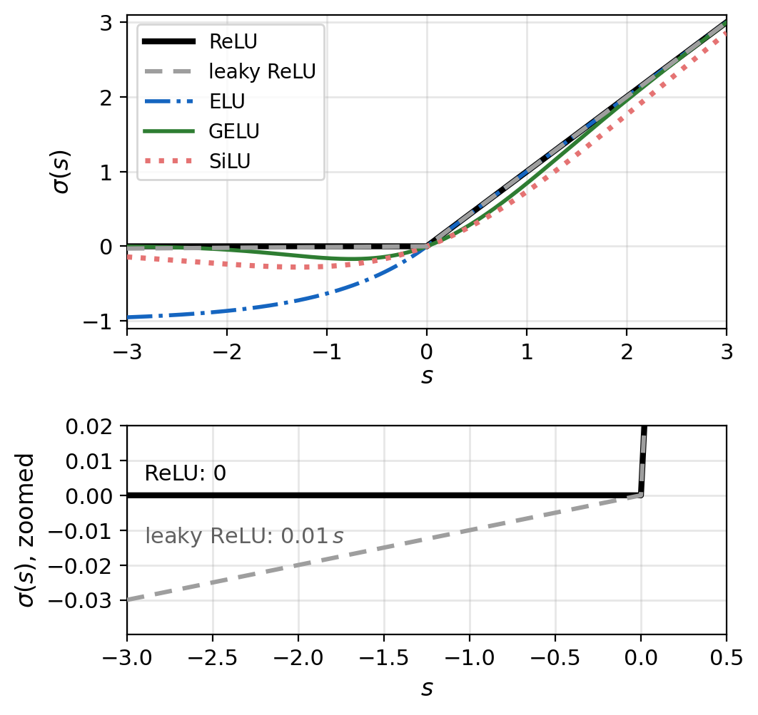
ReLU Variants Give Negative Inputs a Nonzero Slope
Same as ReLU for large positive \(s\), different for \(s < 0\)
- Leaky ReLU: \(0.01\, s\), slope \(0.01\)
- ELU: \(e^{s} - 1\), bounded below by \(-1\)
- GELU: \(s\, \Phi(s)\), \(\Phi\) the standard normal distribution function
- SiLU: \(s \cdot \mathrm{sigmoid}(s)\)
No unit has slope exactly \(0\) on every input
Backward factor at \(v = 0.1,\ 1,\ 10\)
- Leaky ReLU: \(0.50\) at every \(v\), since it also scales: \((1 + 0.01^2)/2\)
- ELU: \(0.82\), \(0.67\), \(0.56\)
- GELU: \(0.30\), \(0.46\), \(0.51\)
- SiLU: \(0.27\), \(0.38\), \(0.50\)
Cost per element, one CPU thread
- Leaky ReLU: the same as ReLU
- ELU, GELU, SiLU: \(2\) to \(6\) times ReLU, from the exponential or the error function
In PyTorch, one module changes
act = nn.GELU      # nn.ReLU, nn.LeakyReLU, nn.ELU, nn.SiLU
net = nn.Sequential(nn.Flatten(), nn.Linear(784, 256), act(),
                    nn.Linear(256, 256), act(), nn.Linear(256, 10))