Training Deep Networks
EE 541 - Unit 7B
Two Moons Overlap, So No Boundary Classifies Every New Point
Data model, class \(c \in \{0, 1\}\)
- A point \(\mathbf{a}_c(t)\) on the class’s half-circle, \(t\) uniform on \([0, \pi]\)
- Plus Gaussian noise of standard deviation \(0.35\)
\[p(\mathbf{x} \mid c) = \frac{1}{\pi}\int_0^{\pi} \mathcal{N}\big(\mathbf{x};\, \mathbf{a}_c(t),\, 0.35^2\,\mathbf{I}\big)\, dt\]
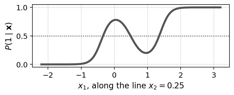
Bayes rule, equal priors: decide class \(1\) where
\[P(1 \mid \mathbf{x}) = \frac{p(\mathbf{x} \mid 1)}{p(\mathbf{x} \mid 0) + p(\mathbf{x} \mid 1)} > \tfrac{1}{2}\]
Training set: \(200\) points, \(100\) per class
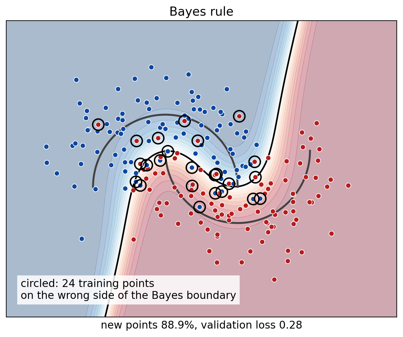
Best accuracy on new points: \(88.9\%\), the Bayes rule’s
- \(24\) of the \(200\) training points lie on its wrong side
Training Accuracy Exceeds the Bayes Accuracy
Training
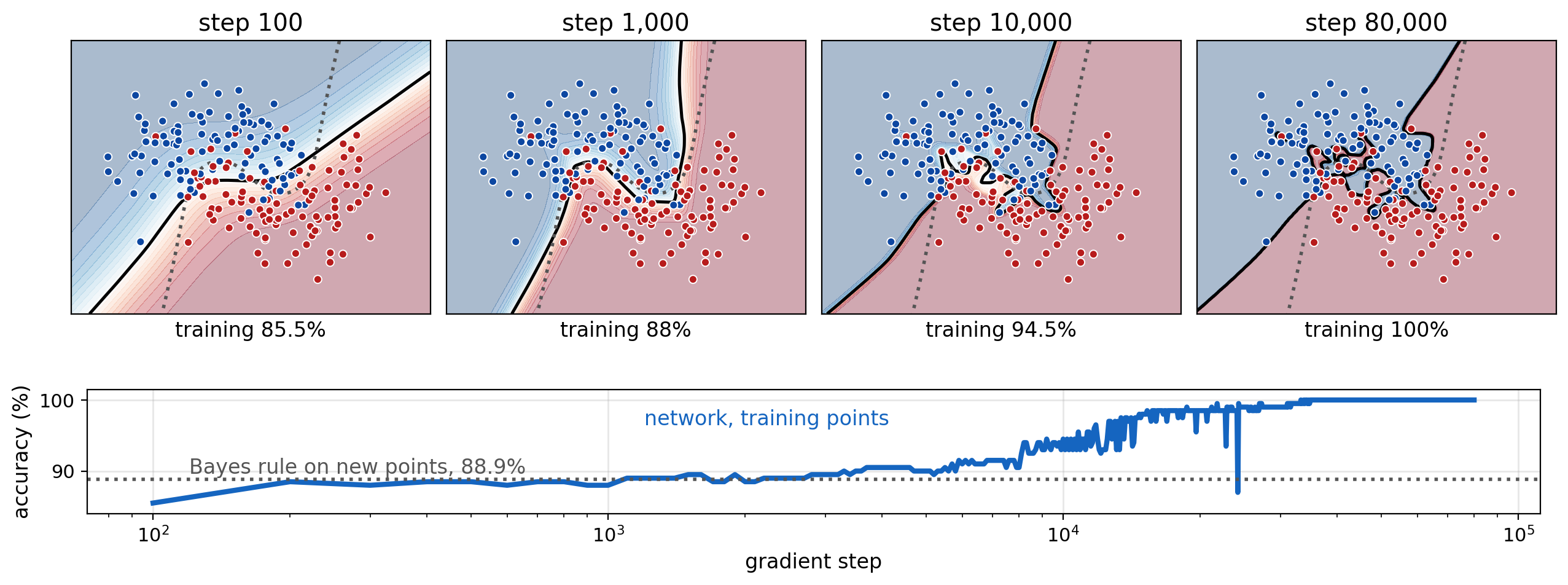
- Two hidden layers of \(256\) ReLU units
- Gradient descent on the average cross-entropy of all \(200\) points, \(\eta = 0.1\)
Past \(88.9\%\): the network fits points that no rule classifies correctly on new data
- \(100\%\) includes the \(24\) points the Bayes rule gets wrong
But Loss on New Points Rises
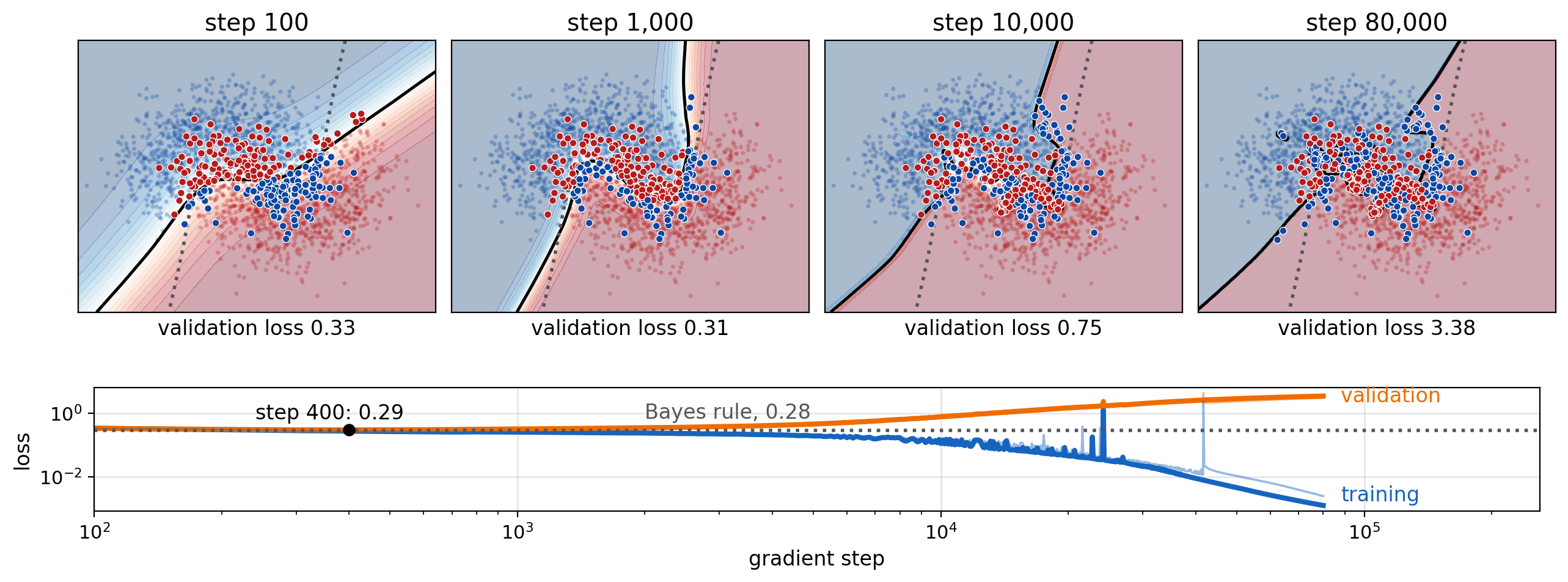
Validation set: \(2{,}000\) new points from the same distribution
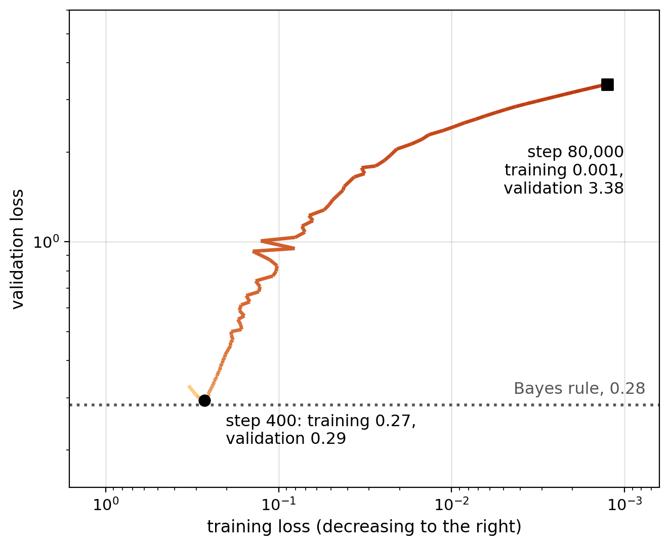
Step \(400\): validation loss \(0.29\), against \(0.28\) for the Bayes rule
After step \(400\): every step lowers the training loss and raises the validation loss
- \(3.38\) at step \(80{,}000\), more than \(10\) times the lowest
Larger Weights Push Probabilities Toward 0 or 1
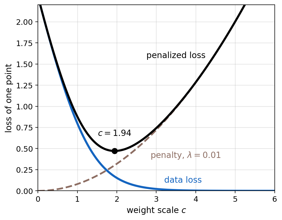
Correctly classified point: logits \(\mathbf{s}\), true class \(y\), margins \(s_y - s_k > 0\)
\[\ell(c\,\mathbf{s}) = \log\Big(1 + \sum_{k \ne y} e^{-c\,(s_y - s_k)}\Big)\]
- Decreasing in \(c\): same decision, smaller loss
- Margin \(2\) to nine other classes: \(0.80\) at \(c = 1\), \(0.15\) at \(c = 2\), \(0.003\) at \(c = 4\)
Every training point correct
- No finite minimizer, as for logistic regression on separable data
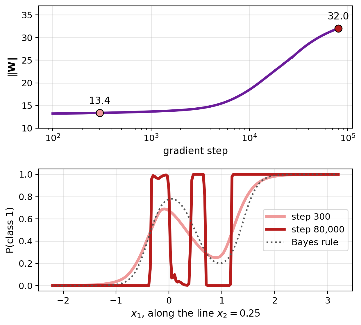
- The weights grow at every step
- Logits grow on every input, new points included
The Network Is Confidently Wrong on New Images
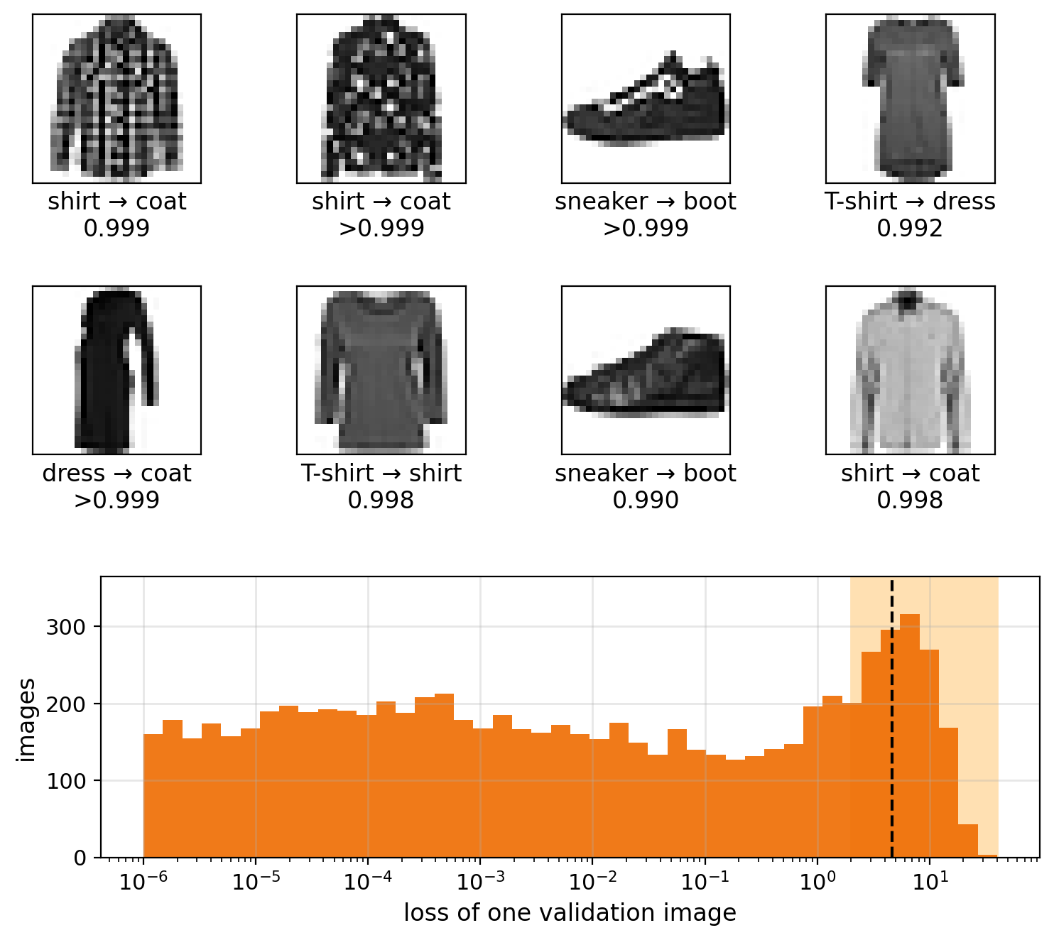
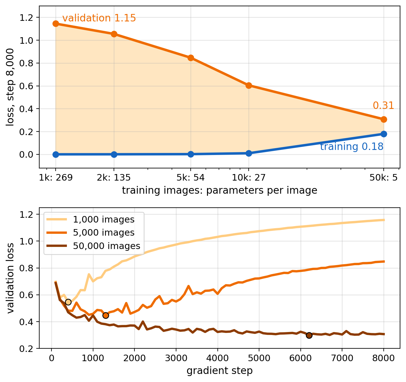
FashionMNIST, \(1{,}000\) training images
- Two hidden layers of \(256\) ReLU units
- \(100\%\) training accuracy
- Lowest validation loss: \(0.55\)
- After \(8{,}000\) steps: \(1.16\)
Wrong with probability above \(0.99\): 620 of the \(10{,}000\) validation images
- Each costs more than \(-\log 0.01 = 4.6\)
Loss above \(2\)
- \(15\%\) of the validation images
- \(92\%\) of the validation loss
The Network Also Fits Randomly Shuffled Labels
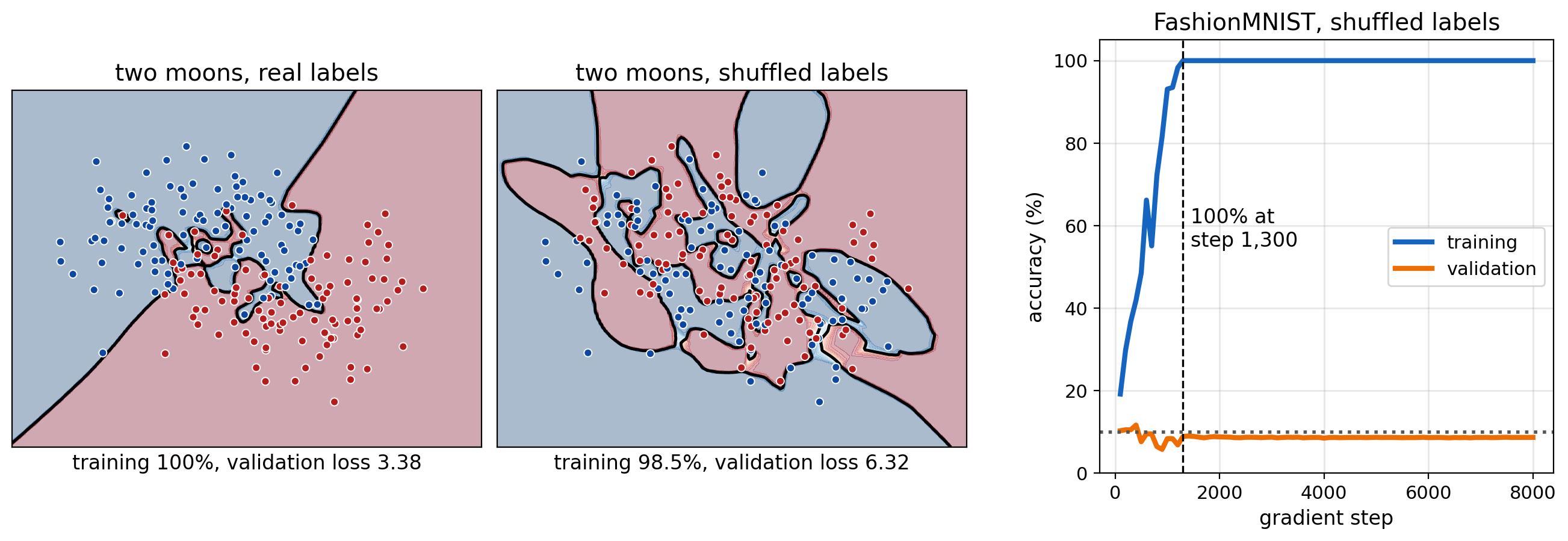
Shuffled labels: a point’s label says nothing about the point
- Two moons: \(98.5\%\) training accuracy, \(50\%\) validation accuracy
- FashionMNIST: \(100\%\) training accuracy, \(9\%\) validation accuracy
Training accuracy reaches nearly \(100\%\) with or without a pattern in the labels
- Only held-out data tell learned classes from stored labels
A Larger Training Set Narrows the Gap
FashionMNIST, the same network and \(8{,}000\) steps
- \(1{,}000\) to \(50{,}000\) training images
Validation loss falls: \(1.15\) at \(1{,}000\) images, \(0.31\) at \(50{,}000\)
- \(269\) parameters per image at \(1{,}000\), \(5\) at \(50{,}000\)
Training loss rises: below \(0.001\) at \(1{,}000\) images, \(0.18\) at \(50{,}000\)
- \(8{,}000\) steps no longer fit every training image
Validation accuracy: \(80\%\), \(85\%\), \(89\%\) at \(1{,}000\), \(5{,}000\), \(50{,}000\)
Lowest validation loss: later and lower with more images
- \(0.55\) at step \(400\) with \(1{,}000\) images
- \(0.30\) at step \(6{,}200\) with \(50{,}000\)
Training Minimizes the Wrong Loss
Training loss, the average over the \(n\) training points
\[\hat{R}_n(f) = \frac{1}{n}\sum_{i=1}^{n} \ell(y_i, f(\mathbf{x}_i))\]
Loss on new data, the expected loss
\[R(f) = \mathbb{E}\big[\ell(Y, f(\mathbf{X}))\big]\]
Fitted network \(\hat{f}_n = \arg\min_f \hat{R}_n(f)\)
- \(\hat{R}_n(\hat{f}_n)\) falls below \(R(\hat{f}_n)\)
- Validation loss: an unbiased estimate of \(R(\hat{f}_n)\)
Two moons, one run
- Lowest training loss: step \(80{,}000\)
- Lowest validation loss: step \(400\)
The L2 Penalty Gives the Loss a Finite Minimizer
Penalized loss, weights only, biases unpenalized
\[\mathcal{L}_\lambda = \frac{1}{n}\sum_{i=1}^{n} \ell_i + \frac{\lambda}{2}\sum_l \|\mathbf{W}^{(l)}\|_F^2\]
- MAP estimate with independent \(\mathcal{N}(0, \tau^2)\) weights, \(\lambda = 1/(n\tau^2)\)
- \(n = 200\), \(\lambda = 0.01\): \(\tau = 0.71\)
Gradient step
\[\mathbf{W} \leftarrow (1 - \eta\lambda)\,\mathbf{W} - \eta\, \nabla_{\mathbf{W}} \frac{1}{n}\sum_i \ell_i\]
- Every weight shrinks by \(1 - \eta\lambda\) before the data step
- \(\eta = 0.1\), \(\lambda = 0.01\): a factor of \(0.999\)
Weight Decay Bounds the Weights and Smooths the Boundary
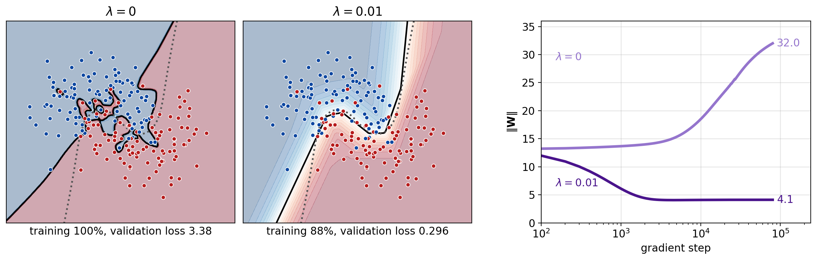
\(\lambda = 0.01\), after \(80{,}000\) steps
- Training accuracy \(88\%\), at the Bayes accuracy of \(88.9\%\)
- Validation loss \(0.296\), against \(0.28\) for the Bayes rule
Without decay: validation loss \(3.38\), weights still growing
With decay: \(\|\mathbf{W}\| = 4.1\) from step \(10{,}000\) on
- The penalty gradient \(\lambda\mathbf{W}\) is equal and opposite to the data gradient
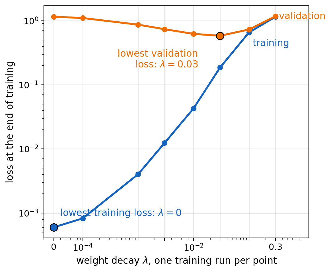
Training Loss Rises With \(\lambda\), Validation Loss Has a Minimum
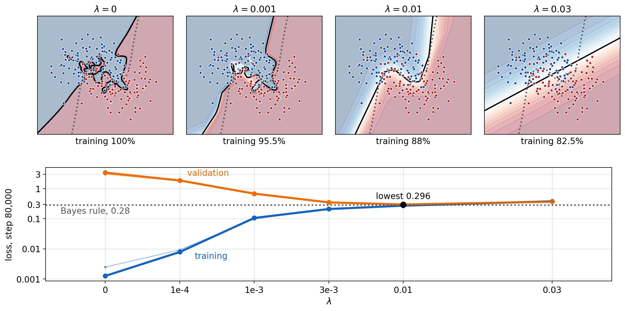
Training loss rises with every increase in \(\lambda\)
- It is lowest at \(\lambda = 0\), the most overfit network
Validation loss has a minimum
- \(3.38\) at \(\lambda = 0\)
- \(0.296\) at \(\lambda = 0.01\), the lowest, with a boundary close to the Bayes boundary
- \(0.37\) at \(\lambda = 0.03\), a nearly straight boundary
- At \(\lambda = 0.03\), training accuracy is below the Bayes accuracy
On FashionMNIST, Weight Decay Removes the Rise in Validation Loss
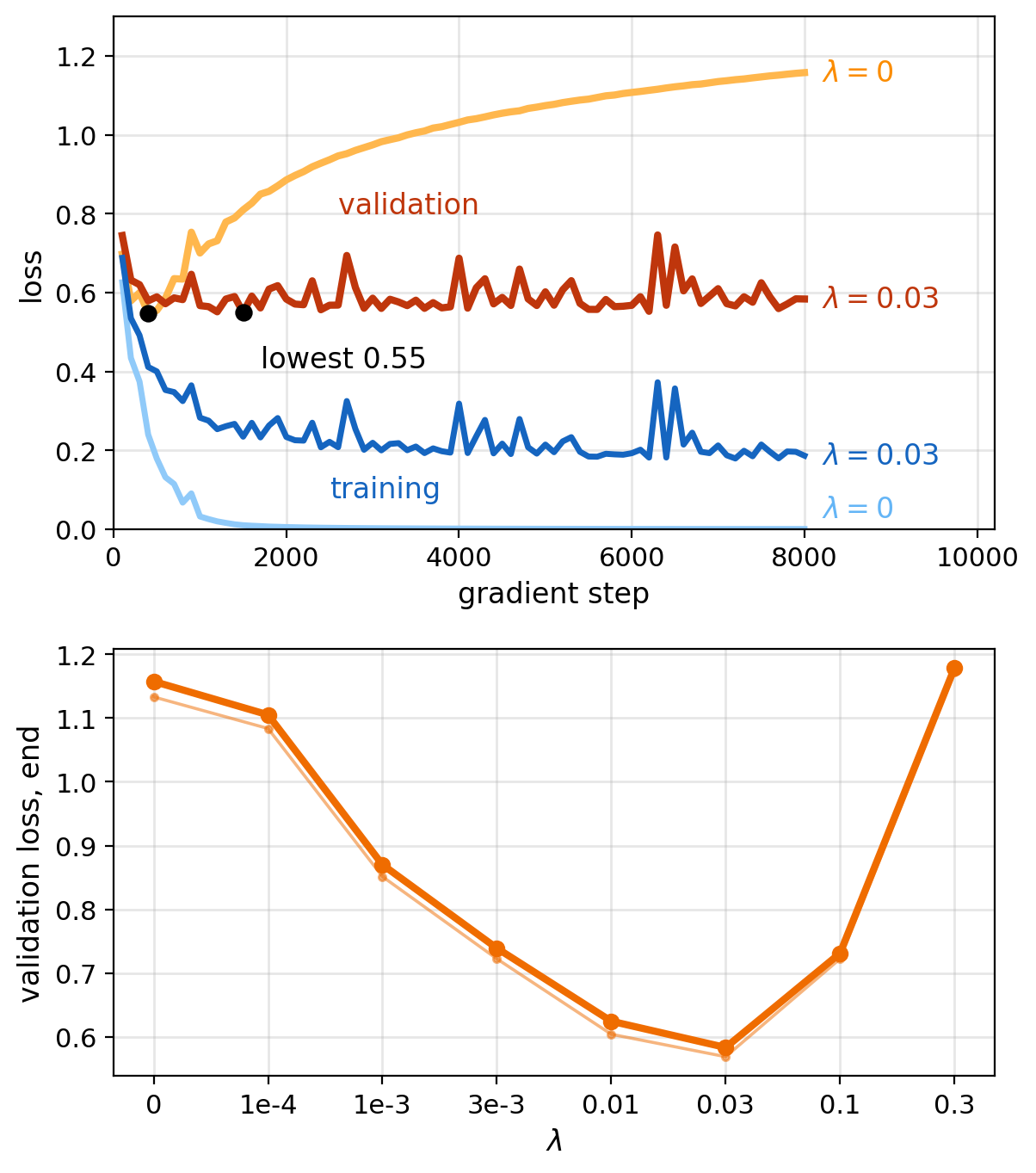
\(1{,}000\) training images, \(8{,}000\) steps
\(\lambda = 0.03\), lowest validation loss at the end
- Validation loss \(0.58\), against \(1.16\) without decay
- Training loss \(0.19\), against \(0.001\)
- Wrong with probability above \(0.99\): 8 images, against 620
- Confidence on wrong predictions: \(0.62\), against \(0.86\)
Validation accuracy: \(80\%\) at both
\(\lambda = 0.3\): validation loss \(1.18\), underfit
Finding the Right \(\lambda\) Takes Many Training Runs
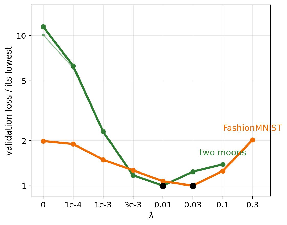
What \(\lambda\) sets: a prior width on the weights, \(\tau = 1/\sqrt{n\lambda}\)
- Two moons, best \(\lambda = 0.01\): \(\tau = 0.71\)
- FashionMNIST, best \(\lambda = 0.03\): \(\tau = 0.18\)
- The right \(\tau\) is not known before training
- One full training run per \(\lambda\) and seed, judged on validation loss
What the penalty depends on: \(\|\mathbf{W}\|\) only, the same for any arrangement of the weights
- It limits how large the weights get, not which units the fit relies on
What it does not change, FashionMNIST
- Lowest validation loss during training: \(0.55\) at every \(\lambda\) up to \(0.03\)
- Weight decay keeps the network near its best point and does not lower it
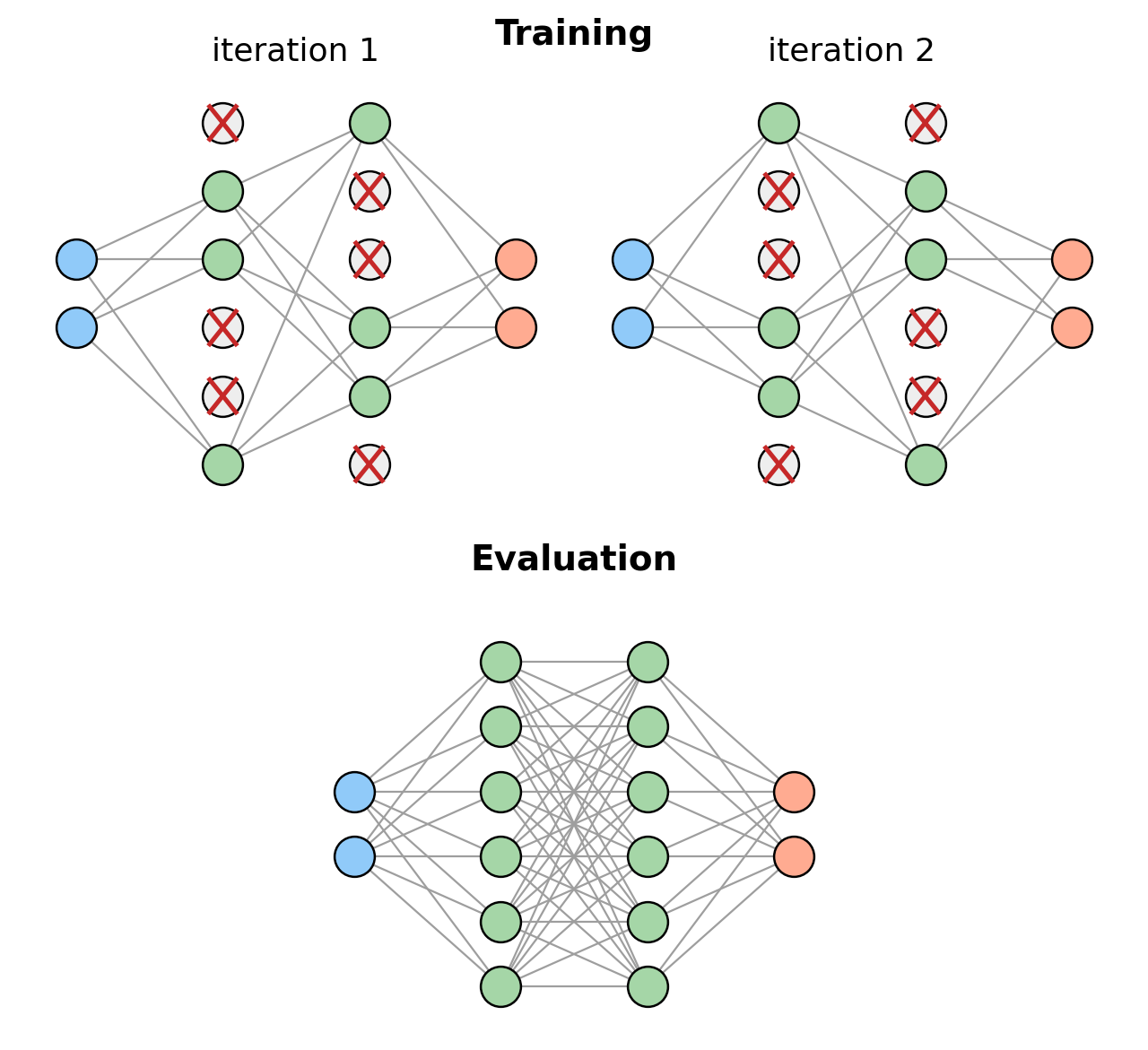
model.eval() Turns Dropout Off
drop = nn.Dropout(p=0.35)
a = torch.tensor([2.0, 0.5, 1.0, 3.0])
drop.train()
print(drop(a))
print(drop(a))      # a new mask each call
drop.eval()
print(drop(a))      # identity
tensor([3.0769, 0.7692, 0.0000, 4.6154])
tensor([0.0000, 0.7692, 1.5385, 4.6154])
tensor([2.0000, 0.5000, 1.0000, 3.0000])Where the scaling happens, the same expected input to the next layer
- Original: no scaling in training, weights times \(1 - p\) at evaluation (Srivastava et al. 2014)
- PyTorch: survivors times \(1/(1 - p)\) in training, nothing at evaluation
Not matched: the variance of the next layer’s input, larger in training than at evaluation
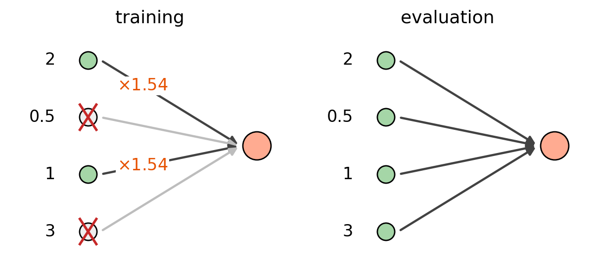
Placement
- After the activation of each hidden layer
- None on the output layer
Rates (Srivastava et al. 2014)
- \(p = 0.5\) on hidden layers
- About \(0.2\) on the input
model = nn.Sequential(
    nn.Linear(784, 1024), nn.ReLU(), nn.Dropout(0.5),
    nn.Linear(1024, 1024), nn.ReLU(), nn.Dropout(0.5),
    nn.Linear(1024, 10))
Evaluating in training mode: a different random subnetwork on every call
Dropout Reduces the Late Rise in Validation Loss
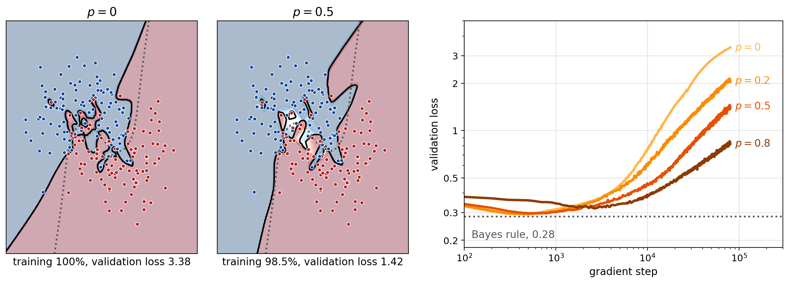
Validation loss after \(80{,}000\) steps
- \(3.38\) without dropout
- \(1.42\) at \(p = 0.5\)
- \(0.82\) at \(p = 0.8\)
Training accuracy: \(100\%\), \(98.5\%\), \(93.5\%\) at \(p = 0, 0.5, 0.8\)
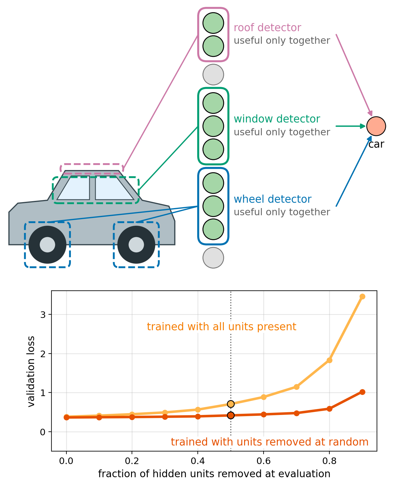
- Fitting a single point takes several specific units
- With dropout, those units are rarely all present on the same step
The Evaluation Network Approximates the Average of the Training Subnetworks
Subnetworks: \(2^n\) masks for \(n\) droppable units, one set of weights
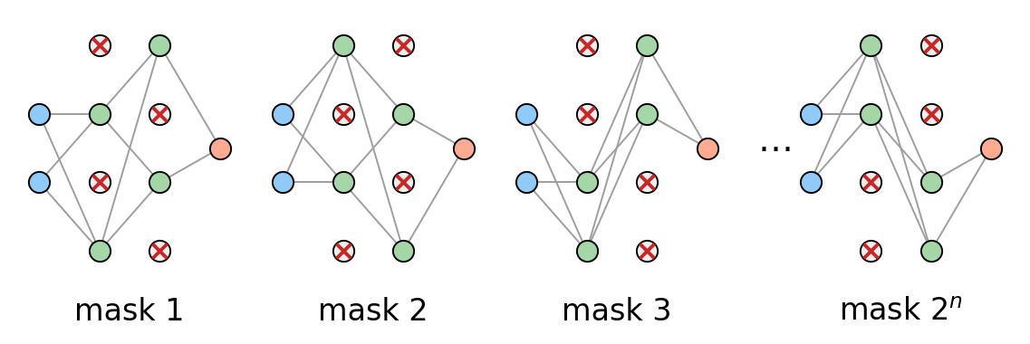
Average prediction over masks \(\mathbf{m}\)
\[\bar{q}(\mathbf{x}) = \mathbb{E}_{\mathbf{m}}\big[q(\mathbf{x}; \mathbf{m})\big]\]
- Exact for a linear layer: scaling by \(1/(1 - p)\) makes the expected input the full network’s input
- Approximate through the nonlinearities
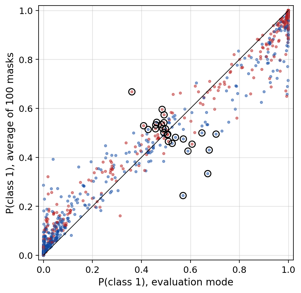
Two moons, \(p = 0.5\)
Evaluation mode against the average of \(100\) random masks
Same predicted class on \(98.7\%\) of the \(2{,}000\) validation points
Dropout Lowers the Best Validation Loss on FashionMNIST
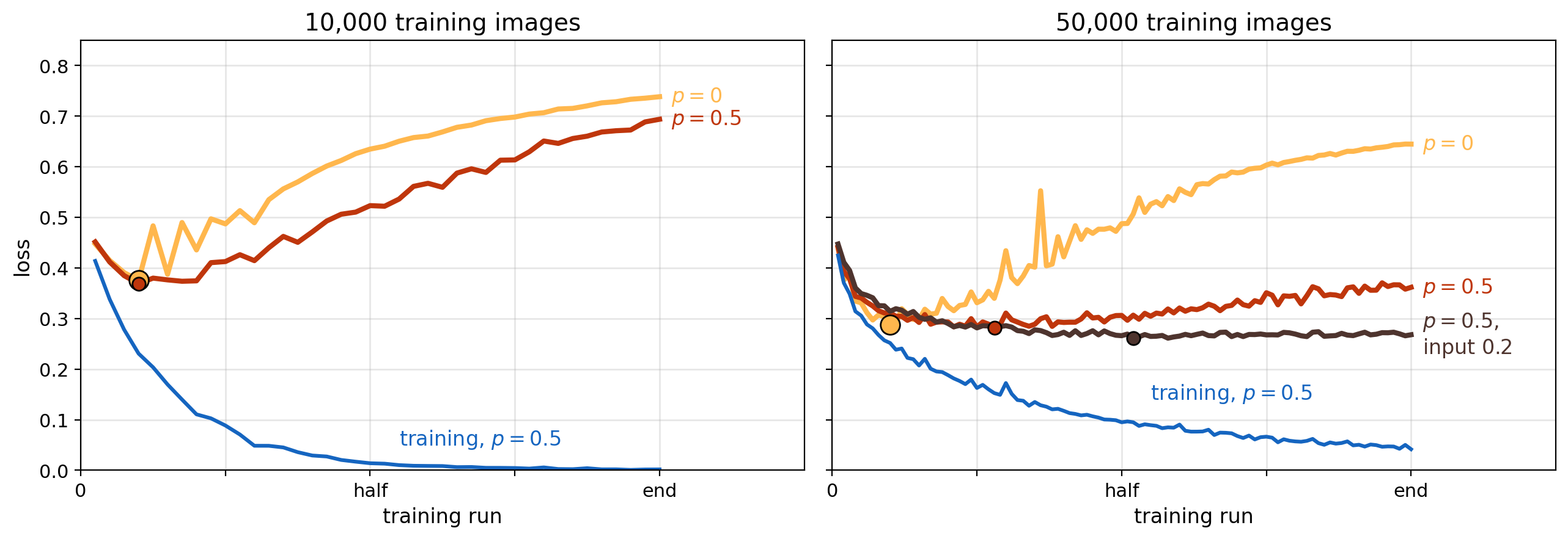
Lowest validation loss
- \(10{,}000\) images: \(0.375\) without dropout, \(0.369\) with
- \(50{,}000\) images: \(0.287\) without, \(0.282\) with
- \(50{,}000\) images, input dropout added: \(0.261\)
Input dropout \(0.2\): a random fifth of the pixels set to \(0\) in each training step
Two hidden layers of \(1{,}024\) units, \(p = 0.5\)
At the end of training
- \(10{,}000\) images: \(0.74\) without, \(0.69\) with
- \(50{,}000\) images: \(0.64\) without, \(0.36\) with
- \(50{,}000\) images, input dropout added: \(0.27\), within \(0.01\) of its lowest
Dropout Does Not Shrink Weights
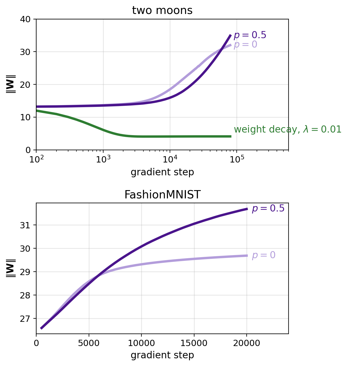
Weight norm \(\|\mathbf{W}\|\), end of training
- Two moons: \(32.0\) without dropout, \(34.9\) with
- Two moons, weight decay \(\lambda = 0.01\): \(4.1\)
- FashionMNIST: \(29.7\) without, \(31.7\) with
Changed by dropout
- Which units the fit relies on
- Validation loss at every step
Unchanged: logits keep growing once the training points are fit
Overtraining Fits Noise
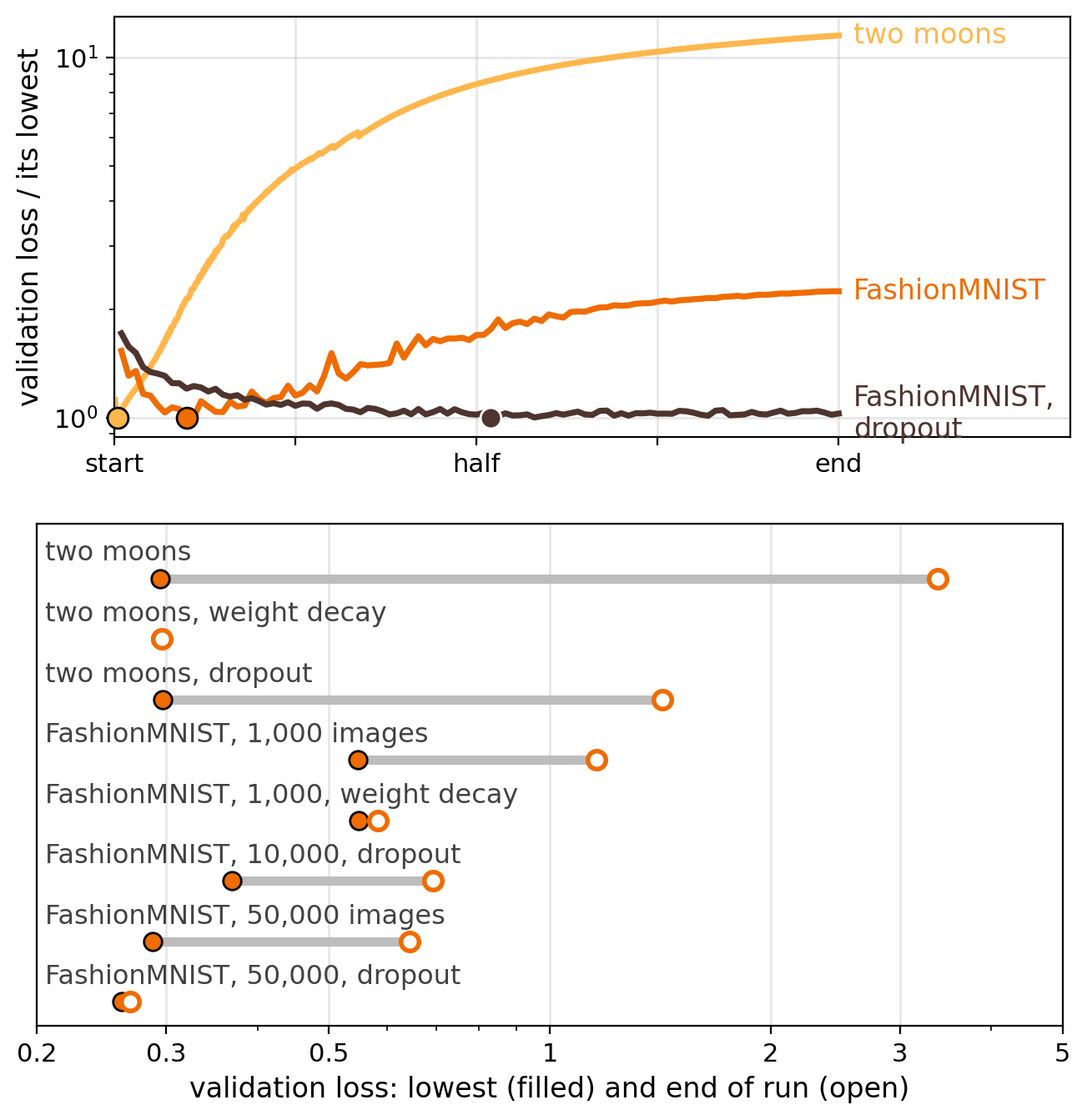
Overtraining: training past the lowest validation loss
Two moons, no regularization
- Training accuracy at step \(80{,}000\): \(100\%\)
- The \(100\%\) includes the \(24\) training points on the wrong side of the Bayes boundary
- Validation loss: \(0.29\) at step \(400\), \(3.38\) at step \(80{,}000\)
FashionMNIST, \(50{,}000\) images, no regularization
- Validation loss: \(0.287\) at epoch \(10\), \(0.64\) at epoch \(100\)
FashionMNIST, \(50{,}000\) images, dropout \(p = 0.5\), input dropout \(0.2\)
- Validation loss: \(0.261\) at epoch \(52\), \(0.268\) at epoch \(100\)
- Lowest point at epoch \(52\), against \(10\) without dropout
- Rise from the lowest point to epoch \(100\): \(0.007\), against \(0.36\)
Early Stopping Limits Overtraining
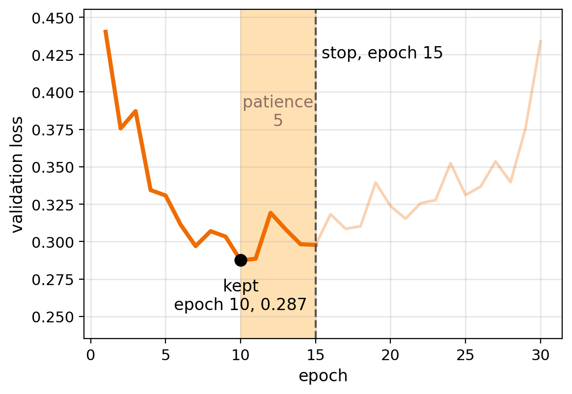
FashionMNIST, \(50{,}000\) images: kept \(0.287\) at epoch \(10\), against \(0.64\) after \(100\) epochs
import copy
best, kept, waited = float('inf'), None, 0
for epoch in range(max_epochs):
    train_one_epoch(model, loader, opt)
    val = val_loss(model, val_loader)  # eval mode
    if val < best:
        best, waited = val, 0
        kept = copy.deepcopy(model.state_dict())
    else:
        waited += 1
        if waited == patience:
            break
model.load_state_dict(kept)
Best network: the parameters with the lowest validation loss of the run
patience: epochs allowed without a new lowest validation lossstate_dict(): the parameters by namecopy.deepcopy:state_dict()returns the live tensors, which later steps change in place- Epochs \(11\) to \(15\) run past the minimum
load_state_dict(kept)restores the epoch-\(10\) parameters
Stopping on a Noisy Validation Loss Needs Patience
Patience \(k\): epochs allowed without a new lowest validation loss
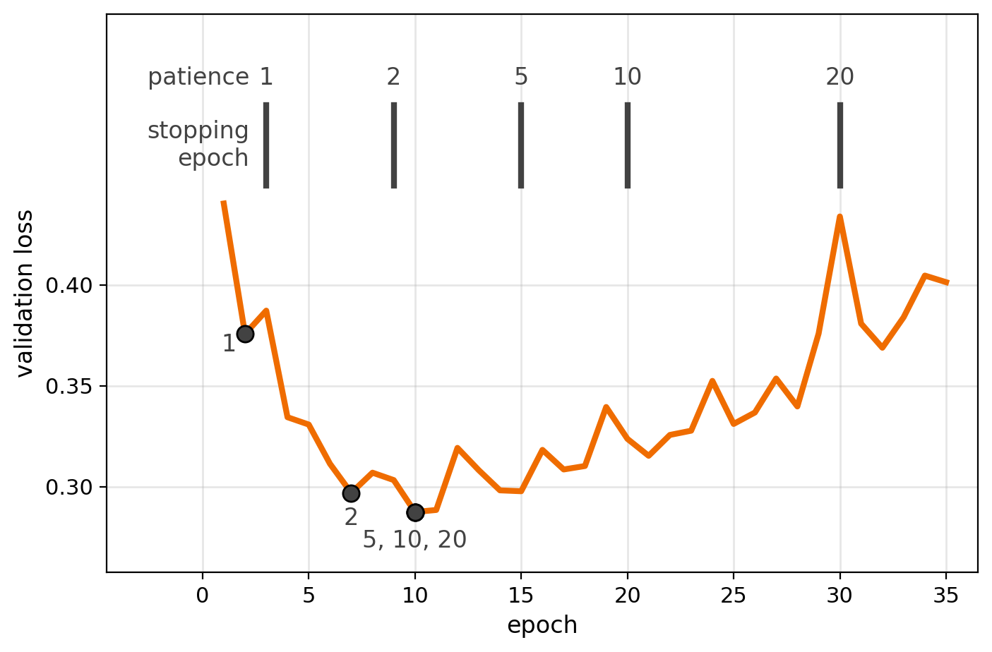
FashionMNIST, \(50{,}000\) images, no regularization
Short patience stops on noise and keeps a worse network
- Patience \(1\): stops at epoch \(3\), keeps \(0.376\)
- Patience \(2\): stops at epoch \(9\), keeps \(0.297\)
Patience \(5\): stops at epoch \(15\)
- Keeps the minimum: epoch \(10\), \(0.287\)
- The same parameters as choosing after all \(100\) epochs
- Stopping saves \(85\) epochs of training
- Kept validation loss: \(0.287\), as after \(100\) epochs
Patience \(20\): the same parameters, \(15\) epochs later
Second seed: patience \(5\) keeps \(0.299\), patience \(10\) the minimum, \(0.291\)
Accuracy Can Stay Level Despite Rising Validation Loss
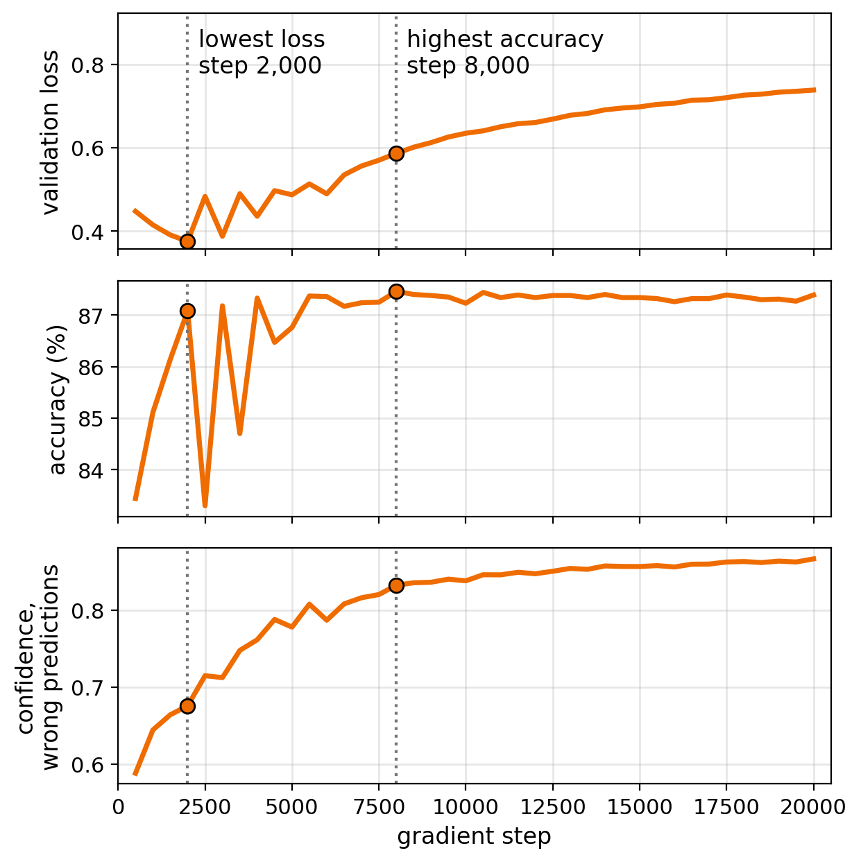
FashionMNIST, \(10{,}000\) images, no regularization
Confidence on wrong predictions: the probability of the predicted class, averaged over misclassified images
From the lowest loss to the end, step \(2{,}000\) to \(20{,}000\)
- Validation loss: \(0.375\) to \(0.738\)
- Accuracy: \(87.1\%\) to \(87.4\%\)
- Confidence on wrong predictions: \(0.68\) to \(0.87\)
Highest accuracy: step \(8{,}000\), \(87.5\%\), validation loss \(0.586\)
Second seed: lowest loss at step \(2{,}500\), highest accuracy at \(9{,}000\)
Kept copy: one per quantity monitored
state = model.state_dict()
if val < best_val:
    best_val, kept_val = val, copy.deepcopy(state)
if acc > best_acc:
    best_acc, kept_acc = acc, copy.deepcopy(state)
Stopping After \(t\) Steps Acts as an L2 Penalty With \(\lambda \approx 1/(\eta t)\)
Early stopping, logistic regression, from \(\mathbf{w} = \mathbf{0}\)
- \(\|\mathbf{w}\|\) grows with the number of steps
- The step count is tuned in place of \(\lambda\)
Quadratic loss near a minimum \(\mathbf{w}^*\), Hessian \(\mathbf{H}\) with eigenvalues \(h_i\), \(w_i\) the component along eigenvector \(i\)
\[\mathcal{L}(\mathbf{w}) = \mathcal{L}(\mathbf{w}^*) + \tfrac{1}{2}(\mathbf{w} - \mathbf{w}^*)^T \mathbf{H}\, (\mathbf{w} - \mathbf{w}^*)\]
Gradient descent from \(\mathbf{w}^{(0)} = \mathbf{0}\), with \(0 < \eta h_i < 1\)
\[\mathbf{w}^{(t)} - \mathbf{w}^* = (\mathbf{I} - \eta \mathbf{H})(\mathbf{w}^{(t-1)} - \mathbf{w}^*) \quad\Rightarrow\quad w_i^{(t)} = \big(1 - (1 - \eta h_i)^t\big)\, w_i^*\]
L2 penalty \(\tfrac{\lambda}{2}\|\mathbf{w}\|^2\)
\[\mathbf{H}(\mathbf{w} - \mathbf{w}^*) + \lambda \mathbf{w} = \mathbf{0} \quad\Rightarrow\quad w_i = \frac{h_i}{h_i + \lambda}\, w_i^*\]
From a random start \(\mathbf{w}^{(0)}\): \(\mathbf{w} - \mathbf{w}^{(0)}\) in place of \(\mathbf{w}\), so the penalty is \(\tfrac{\lambda}{2}\|\mathbf{w} - \mathbf{w}^{(0)}\|^2\)
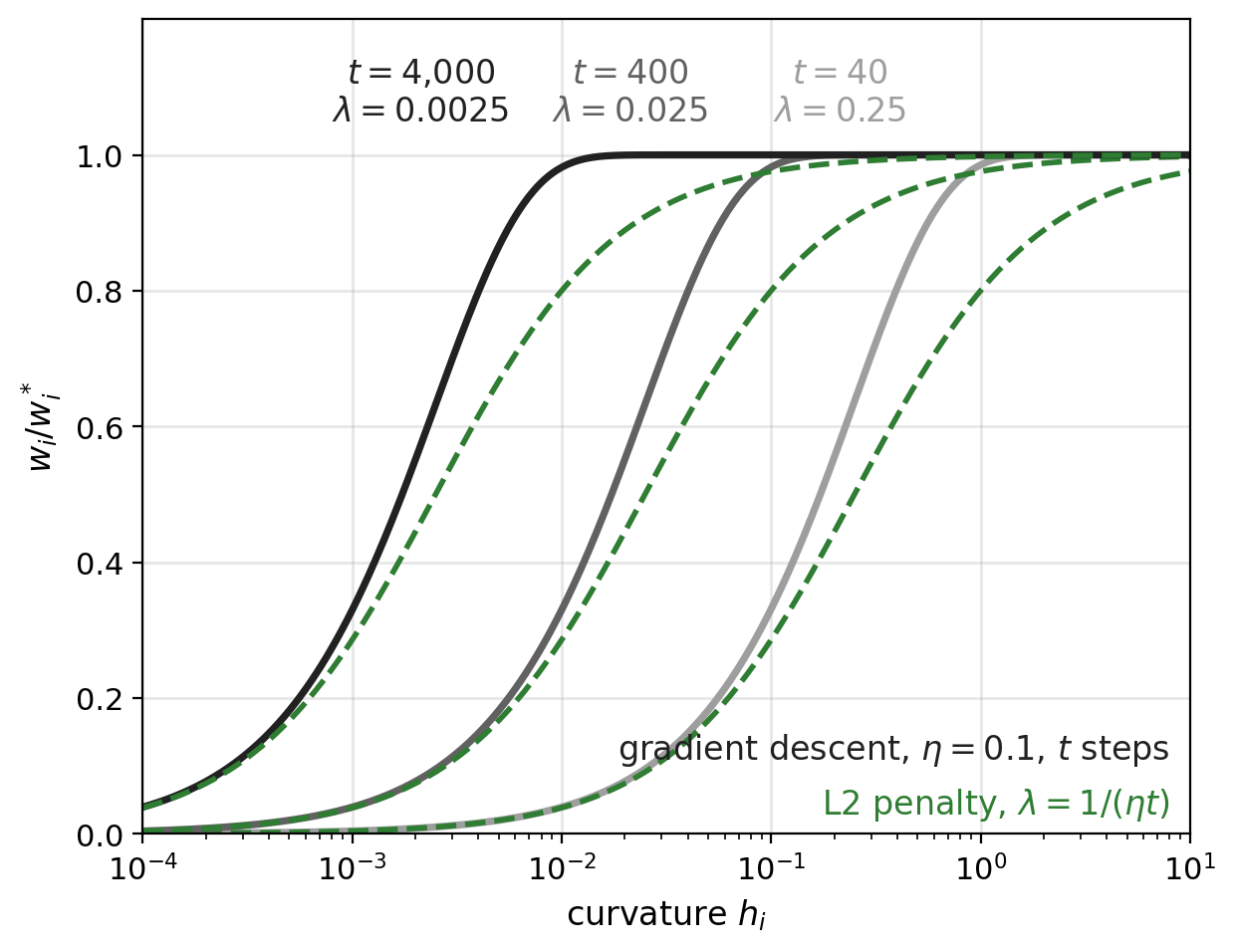
Both factors are near \(1\) where \(h_i\) is large and near \(0\) where \(h_i\) is small
\[\eta h_i t \ll 1: \qquad \eta h_i t \;\approx\; \frac{h_i}{\lambda} \quad\Rightarrow\quad \lambda = \frac{1}{\eta t}\]
Early Stopping Regularizes Toward the Initial Weights
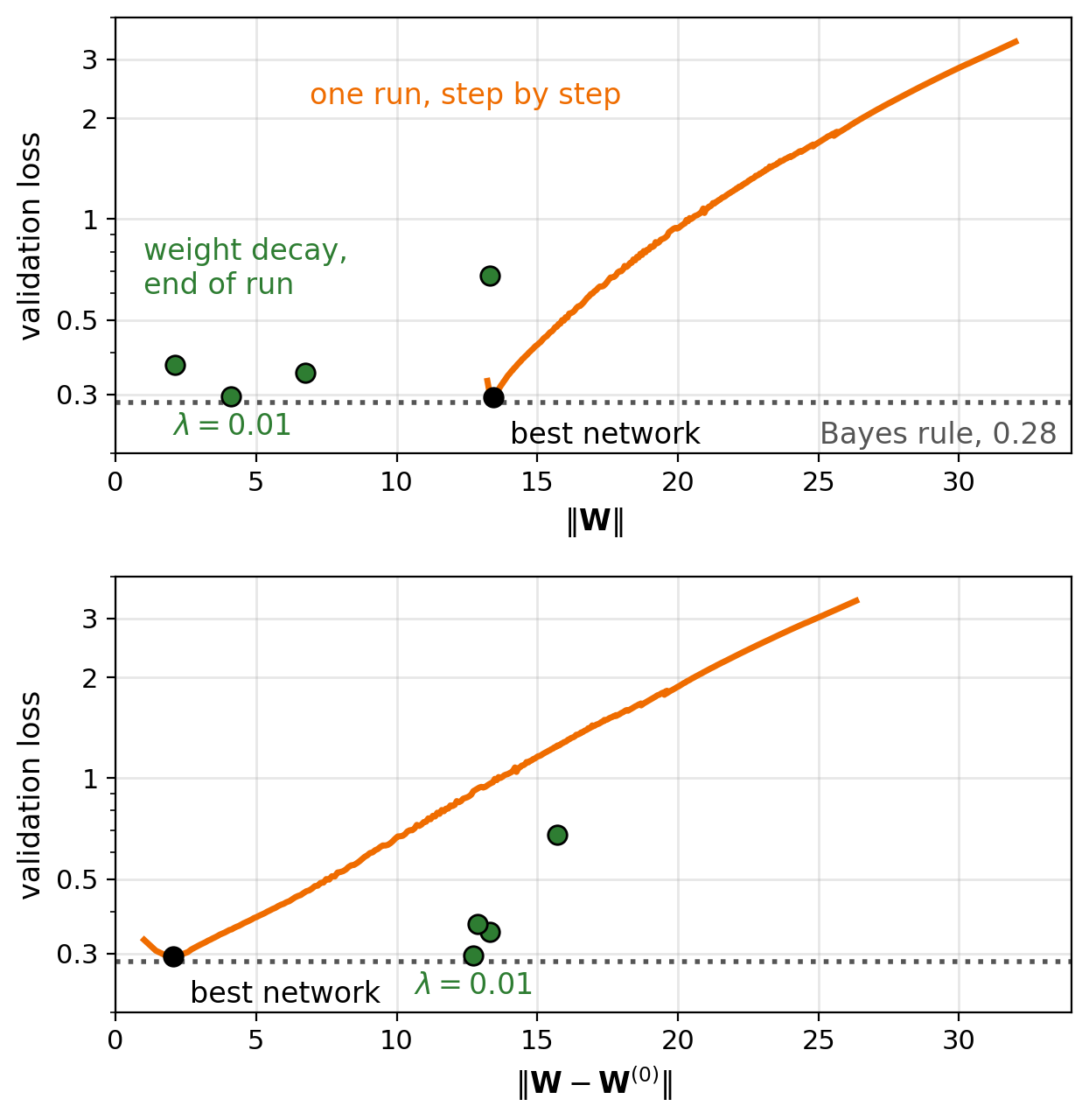
\(\|\mathbf{W}\|\): the norm of all weight matrices, biases excluded
Two moons, one run without regularization
- Start: \(\|\mathbf{W}^{(0)}\| = 13.1\)
- Best step, \(400\): \(\|\mathbf{W} - \mathbf{W}^{(0)}\| = 2.05\), \(\|\mathbf{W}\| = 13.4\)
- Step \(80{,}000\): \(\|\mathbf{W} - \mathbf{W}^{(0)}\| = 26.3\)
Weight decay, \(\lambda = 0.01\): a penalty centered at \(\mathbf{0}\)
- After \(80{,}000\) steps: \(\|\mathbf{W}\| = 4.1\), \(\|\mathbf{W} - \mathbf{W}^{(0)}\| = 12.7\)
Validation loss, Bayes rule \(0.28\) (computed from the generating distribution)
- Early stopping: \(0.29\)
- Weight decay: \(0.296\)
When to Stop Training Depends on the Learning Rate
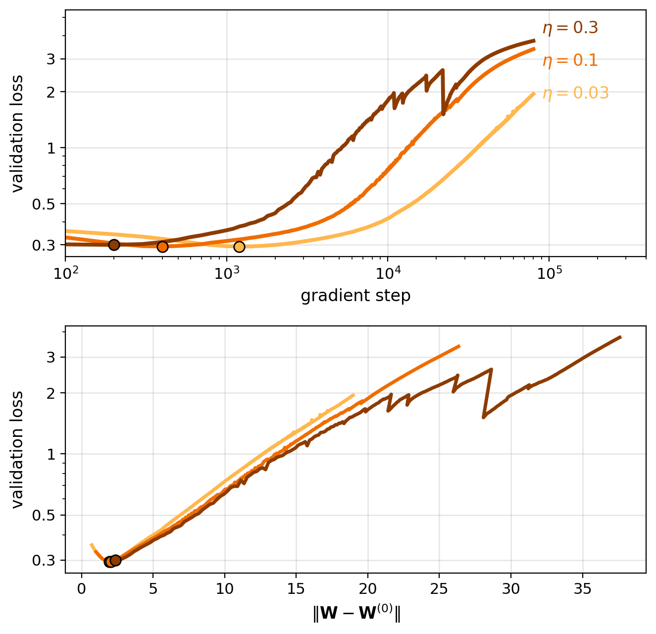
Two moons, the same network, data, and start, three learning rates
Best stopping step, full batch: one step per epoch
- \(\eta = 0.03\): step \(1{,}200\)
- \(\eta = 0.1\): step \(400\)
- \(\eta = 0.3\): step \(200\)
Best network at every \(\eta\)
- \(\|\mathbf{W} - \mathbf{W}^{(0)}\| = 2.0\) to \(2.4\)
- Validation loss \(0.29\) to \(0.30\)
- \(\eta t = 36\), \(40\), \(60\), with validation loss evaluated every \(100\) steps
A stopping step tuned at one \(\eta\): not the best step at any other \(\eta\)
- With \(\eta_k\) changing from step to step, \(\sum_k \eta_k\) takes the place of \(\eta t\)
Label Smoothing Replaces Hard Targets With Soft Targets
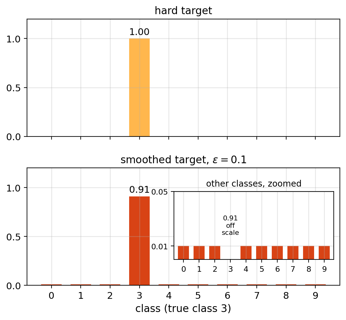
Hard target: one-hot, \(1\) on the true class and \(0\) on every other class
Label smoothing: a fraction \(\varepsilon\) of the target moved off the true class and spread evenly over all \(K\) classes
\[\tilde{y}_k = (1 - \varepsilon)\, y_k + \frac{\varepsilon}{K}\]
- \(K = 10\), \(\varepsilon = 0.1\): \(1\) becomes \(0.91\), each \(0\) becomes \(0.01\)
- \(K = 2\), \(\varepsilon = 0.1\): \(1\) becomes \(0.95\), \(0\) becomes \(0.05\)
Soft target: a probability distribution over the classes, which CrossEntropyLoss accepts as a target
- Here the same for every example of a class
- The same value on every other class
One-Hot Cross-Entropy Has No Finite Best Logit Gap
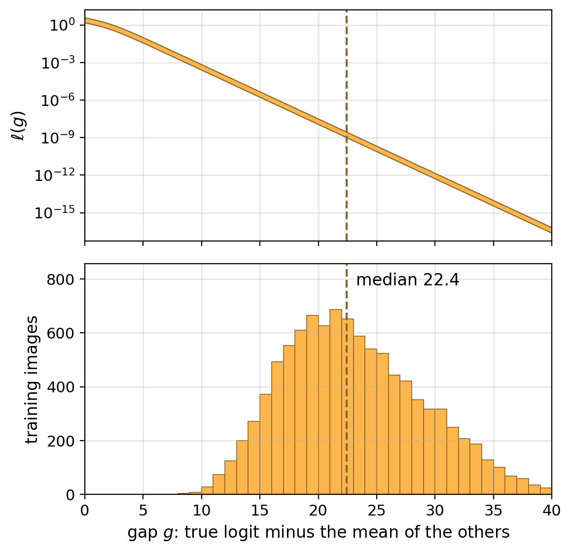
Cross-entropy with a hard target, true logit ahead of each of the other \(K - 1\) logits by \(g\)
\[\ell(g) = \log\big(1 + (K - 1)\, e^{-g}\big)\]
- Falls at every \(g\): with every training point correct, no finite minimizer
FashionMNIST, \(10{,}000\) images, two hidden layers of \(1{,}024\) units, \(20{,}000\) steps
- Training accuracy: \(100\%\)
- Gap \(g\), true logit minus the mean of the other nine, median over training images: \(22.4\)
- Loss at that gap: below \(10^{-8}\)
Smoothed Cross-Entropy Has a Finite Best Logit Gap
\(q_k\): the softmax probability of class \(k\)
Loss at gap \(g\), the other logits equal
\[\tilde{\ell}(g) = -\tilde{y}_{\text{true}} \log q_{\text{true}}(g) - (1 - \tilde{y}_{\text{true}}) \log q_{\text{other}}(g)\]
Lowest at \(q = \tilde{y}\)
\[g^* = \log \frac{1 - \varepsilon + \varepsilon/K}{\varepsilon / K}\]
Predicted and measured, median gap over training images
- \(\varepsilon = 0.05\): \(5.25\) and \(5.29\)
- \(\varepsilon = 0.1\): \(4.51\) and \(4.53\)
- \(\varepsilon = 0.2\): \(3.71\) and \(3.72\)
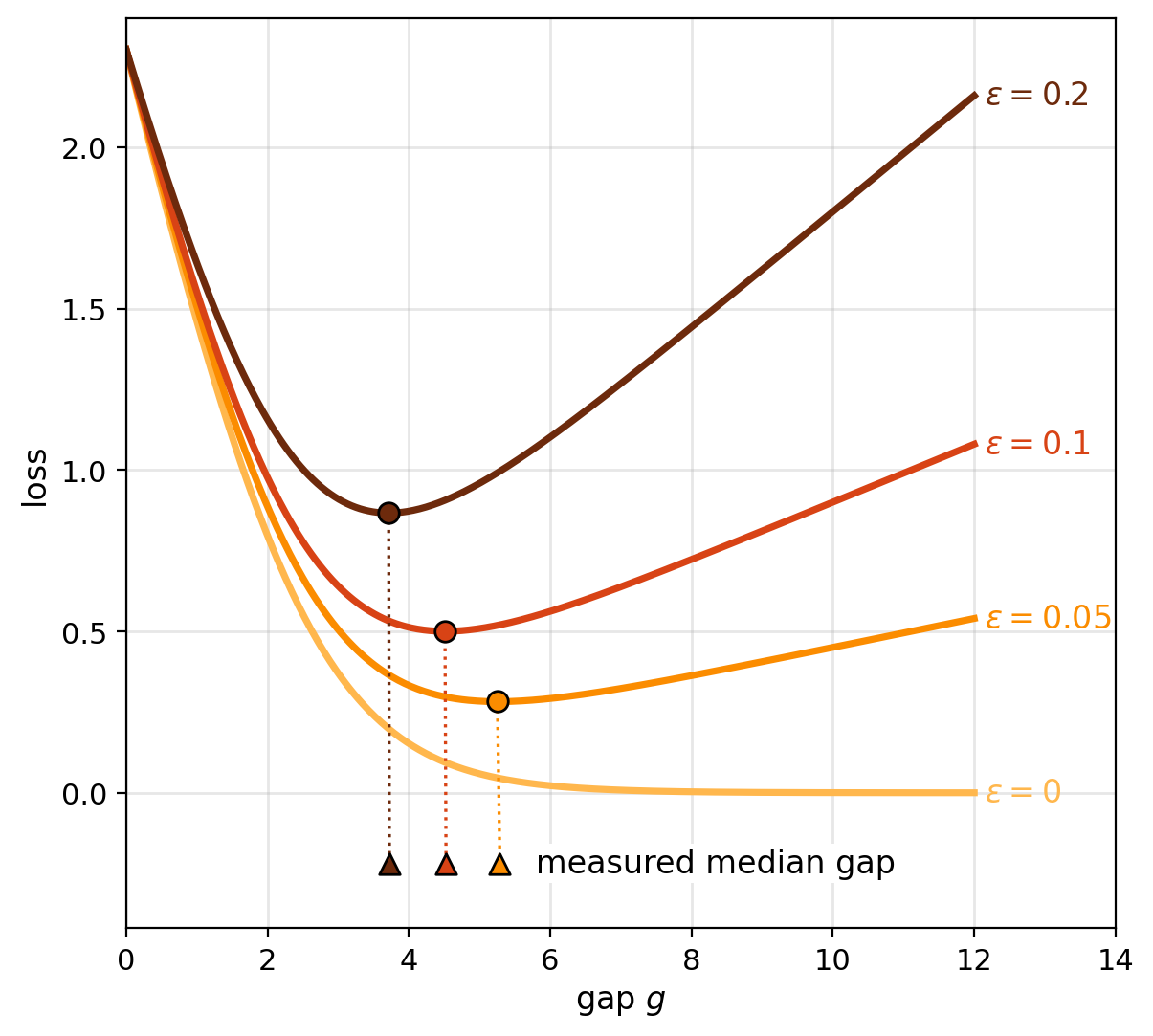
Label Smoothing Reduces Overconfidence
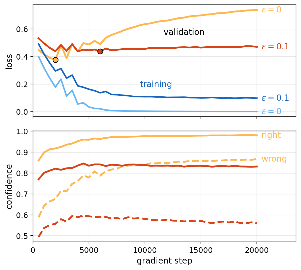
Validation loss: plain cross-entropy against the true labels
Confidence: the largest softmax probability
FashionMNIST, \(10{,}000\) images, \(\varepsilon = 0\) and \(0.1\), end of training
- Validation loss: \(0.738\) and \(0.471\)
- Confidence on wrong predictions: \(0.87\) and \(0.56\)
- Confidence on right predictions: \(0.98\) and \(0.83\)
- Accuracy: \(87.4\%\) and \(87.9\%\)
With \(\varepsilon = 0.1\), validation loss ends within \(0.04\) of its lowest
Lowest validation loss: \(0.375\) and \(0.437\), higher with smoothing
- Floor per correct image at \(\varepsilon = 0.1\): \(-\log 0.91 = 0.094\)
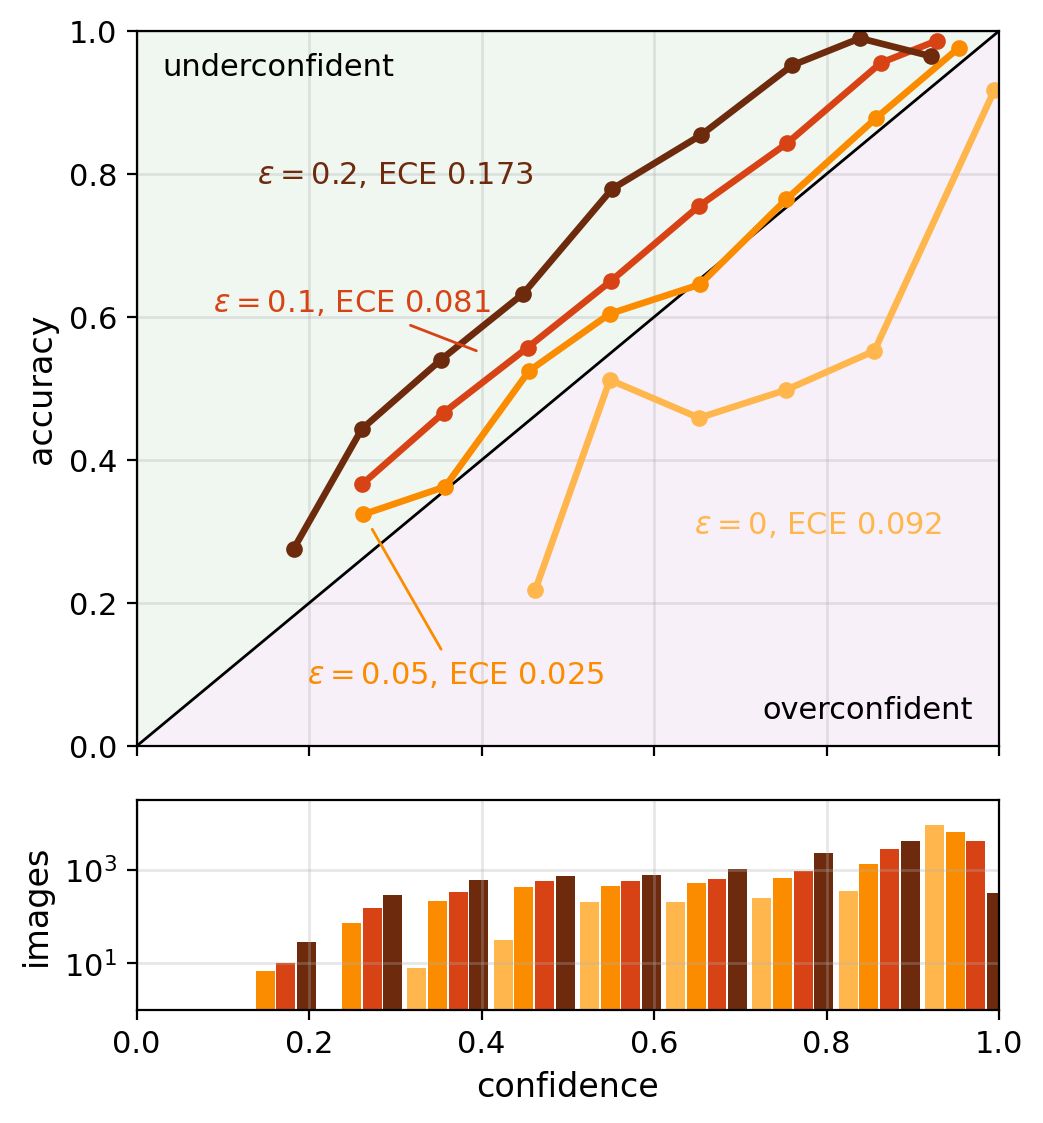
Too Much Smoothing Makes the Network Underconfident
Calibration: among predictions given confidence \(\approx c\), a fraction \(c\) correct
- Overconfident: mean confidence above accuracy
- Underconfident: below
Expected calibration error (ECE): the gap between confidence and accuracy, averaged over \(10\) confidence bins weighted by their counts
FashionMNIST, \(10{,}000\) images, validation set, mean confidence and accuracy
- \(\varepsilon = 0\): \(0.965\) and \(0.874\), ECE \(0.092\)
- \(\varepsilon = 0.05\): \(0.854\) and \(0.878\), ECE \(0.025\)
- \(\varepsilon = 0.1\): \(0.798\) and \(0.879\), ECE \(0.081\)
- \(\varepsilon = 0.2\): \(0.708\) and \(0.881\), ECE \(0.173\)
- Confidence falls with \(\varepsilon\), accuracy barely changes
\(\varepsilon\): a setting chosen on the validation set
Label Smoothing Gives Every Other Class Nearly the Same Logit
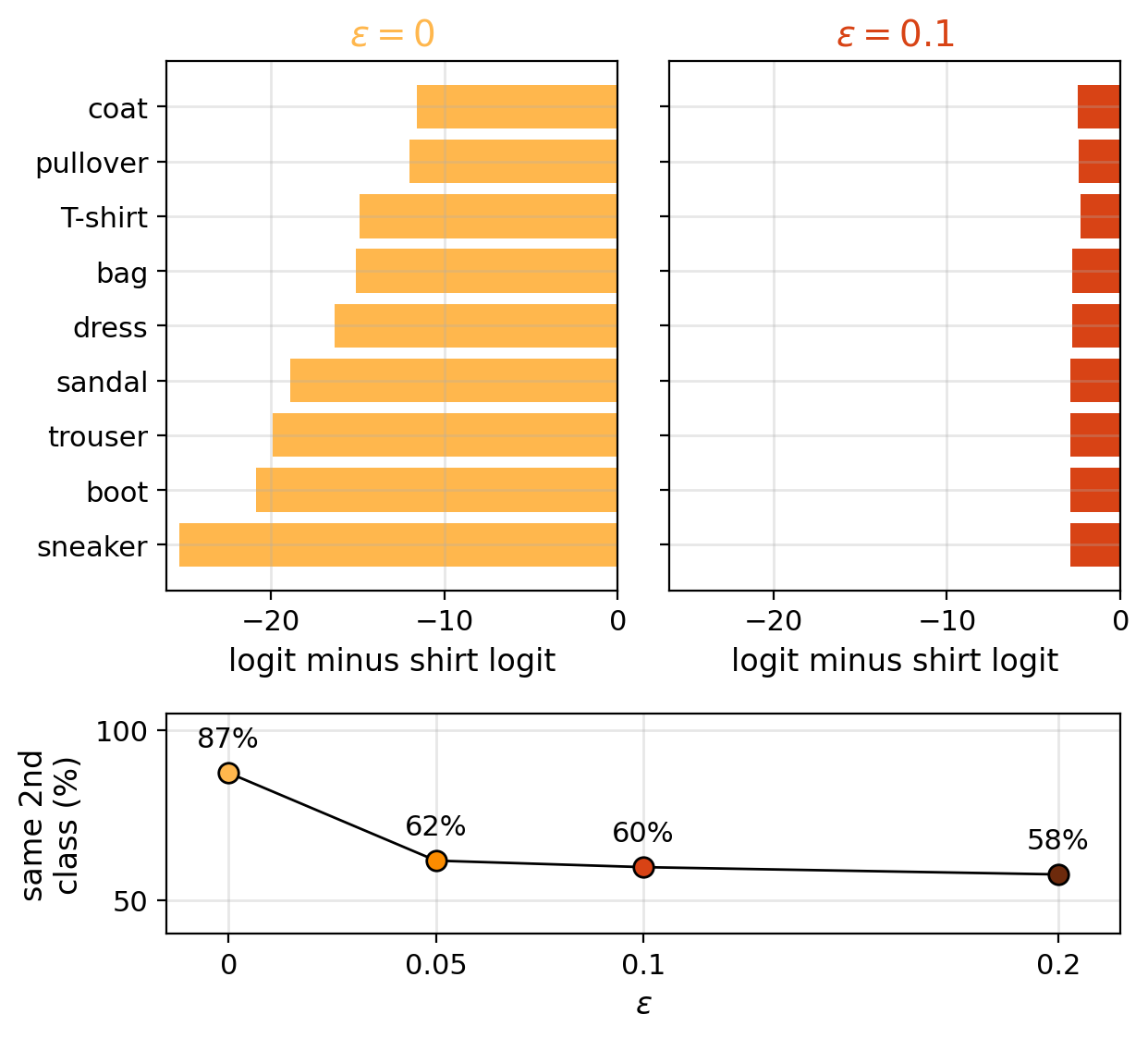
Smoothed target: \(\varepsilon / K\) on every other class, the same for a coat as for a sneaker
Shirt images, mean logit minus the shirt logit
- \(\varepsilon = 0\): coat \(-11.6\), pullover \(-12.0\), T-shirt \(-14.8\), sneaker \(-25.3\)
- \(\varepsilon = 0.1\): \(-2.3\) to \(-2.9\), a range of \(0.6\) against \(13.7\)
Class ranked second, the same in two training runs (seeds \(0\) and \(1\))
- \(\varepsilon = 0\): \(87\%\) of validation images
- \(\varepsilon = 0.1\): \(60\%\)
- With smoothing, the ranking of the other classes is mostly run-to-run noise
Distillation trains on the other classes’ probabilities (Müller et al. 2019)
- A network trained with label smoothing is a weaker teacher
One Learning Rate Moves Some Weights Too Far and Others Too Little
SGD: \(\mathbf{w} \leftarrow \mathbf{w} - \eta\, \mathbf{g}_t\), with \(\mathbf{g}_t\) the minibatch gradient
- One \(\eta\) for every weight
- Step per weight: proportional to its own gradient
Per layer, plain SGD: relative steps differing by orders of magnitude across layers
- Gradient noise: steps that change sign from one minibatch to the next
Two changes to the gradient, before the step
- An average over recent steps: momentum
- A division by each weight’s recent gradient size: Adagrad, RMSprop
- Both: Adam
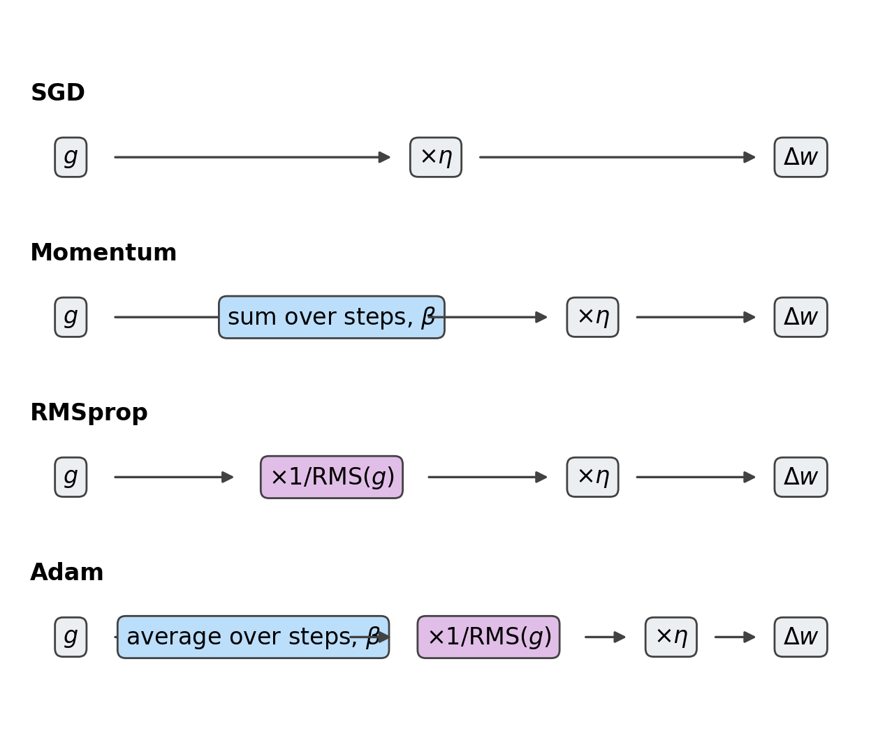
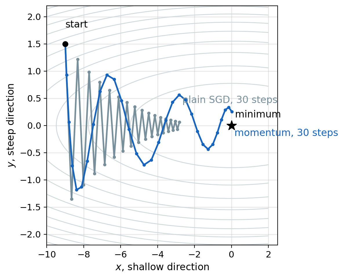
Momentum Cancels Gradient Components That Change Sign
SGD with momentum, PyTorch’s form
\[\mathbf{m}_t = \beta\, \mathbf{m}_{t-1} + \mathbf{g}_t, \qquad \mathbf{w} \leftarrow \mathbf{w} - \eta\, \mathbf{m}_t\]
Unrolled: \(\mathbf{m}_t = \mathbf{g}_t + \beta\, \mathbf{g}_{t-1} + \beta^2 \mathbf{g}_{t-2} + \cdots\)
- A gradient \(10\) steps old: weight \(\beta^{10} = 0.35\) at \(\beta = 0.9\)
- Components that change sign each step: cancel
- Components that keep their sign: add up
Valley, set by hand: steep across (\(\eta < 2/50 = 0.04\) for plain SGD), shallow along
- Plain SGD, \(\eta = 0.038\): oscillates across, small steps along
- Momentum, \(\eta = 0.0076\): effective step \(0.076\) along the valley, beyond plain SGD’s limit across it
Variants: Nesterov, the gradient at the point momentum is about to reach, SGD(nesterov=True)
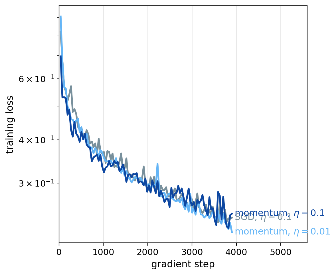
Momentum Raises the Effective Learning Rate to \(\eta / (1 - \beta)\)
Steady gradient \(\mathbf{g}\): \(\mathbf{m}_t \to \mathbf{g}/(1 - \beta)\)
- Step: \(\eta\, \mathbf{g}/(1 - \beta)\)
- \(\beta = 0.9\): ten times plain SGD’s step at the same \(\eta\)
- Adding momentum without lowering \(\eta\): a ten-times-larger effective step
FashionMNIST, two hidden layers of \(256\) units, \(10\) epochs
- Momentum \(0.9\), \(\eta = 0.01\): effective \(0.1\), close to plain SGD at \(\eta = 0.1\)
- Momentum \(0.9\), \(\eta = 0.1\): effective \(1.0\), validation loss at the end \(0.35\) and \(0.37\) (two seeds)
- The other two: \(0.30\) to \(0.32\)
Averaged form: \(\mathbf{m}_t = \beta\, \mathbf{m}_{t-1} + (1 - \beta)\, \mathbf{g}_t\), the same update with \(\eta\) divided by \(1 - \beta\)
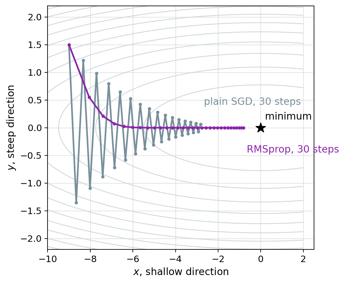
Per-Weight Scaling Gives Steep and Shallow Directions Similar Steps
Per-weight scale: the step divided by an estimate of the gradient’s size, elementwise
- Large, steady gradients: smaller steps
- Small gradients: larger steps
Adagrad: \(\mathbf{s}_t = \mathbf{s}_{t-1} + \mathbf{g}_t^2\), step \(\eta\, \mathbf{g}_t / (\sqrt{\mathbf{s}_t} + \delta)\)
- \(\mathbf{s}_t\) only grows: for a steady gradient the step shrinks as \(1/\sqrt{t}\)
RMSprop: a running average in place of the sum
\[\mathbf{v}_t = \beta_2\, \mathbf{v}_{t-1} + (1 - \beta_2)\, \mathbf{g}_t^2, \qquad \mathbf{w} \leftarrow \mathbf{w} - \eta\, \frac{\mathbf{g}_t}{\sqrt{\mathbf{v}_t} + \delta}\]
- \(\sqrt{\mathbf{v}_t}\): the RMS of the weight’s recent gradients
Valley: similar step sizes across and along
- Steps of fixed size: the path stops short of the minimum without a decaying \(\eta\)
Bias Correction Removes the Start-Up Error of Averages Started at Zero
Adam (Kingma and Ba 2015): momentum as an average, RMSprop’s scale
\[\mathbf{m}_t = \beta_1 \mathbf{m}_{t-1} + (1 - \beta_1)\, \mathbf{g}_t, \qquad \mathbf{v}_t = \beta_2 \mathbf{v}_{t-1} + (1 - \beta_2)\, \mathbf{g}_t^2\]
\[\hat{\mathbf{m}}_t = \frac{\mathbf{m}_t}{1 - \beta_1^t}, \qquad \hat{\mathbf{v}}_t = \frac{\mathbf{v}_t}{1 - \beta_2^t}, \qquad \mathbf{w} \leftarrow \mathbf{w} - \eta\, \frac{\hat{\mathbf{m}}_t}{\sqrt{\hat{\mathbf{v}}_t} + \delta}\]
- \(\mathbf{m}_t\) here: momentum’s sum times \(1 - \beta_1\), an average
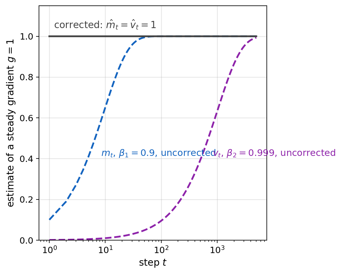
Started at zero, steady gradient \(g\): \(m_t = (1 - \beta_1^t)\, g\), \(v_t = (1 - \beta_2^t)\, g^2\)
- \(v_t\) lags further: \(\beta_2 = 0.999\), half its level after about \(700\) steps
- Uncorrected step at \(t = 1\): \((1 - \beta_1)/\sqrt{1 - \beta_2} = 3.2\,\eta\), too large
Correction: division by \(1 - \beta^t\), exact for a steady gradient
- Defaults: \(\beta_1 = 0.9\), \(\beta_2 = 0.999\), \(\delta = 10^{-8}\), \(\eta = 10^{-3}\)
Adam’s Step Size Does Not Depend on the Gradient’s Scale
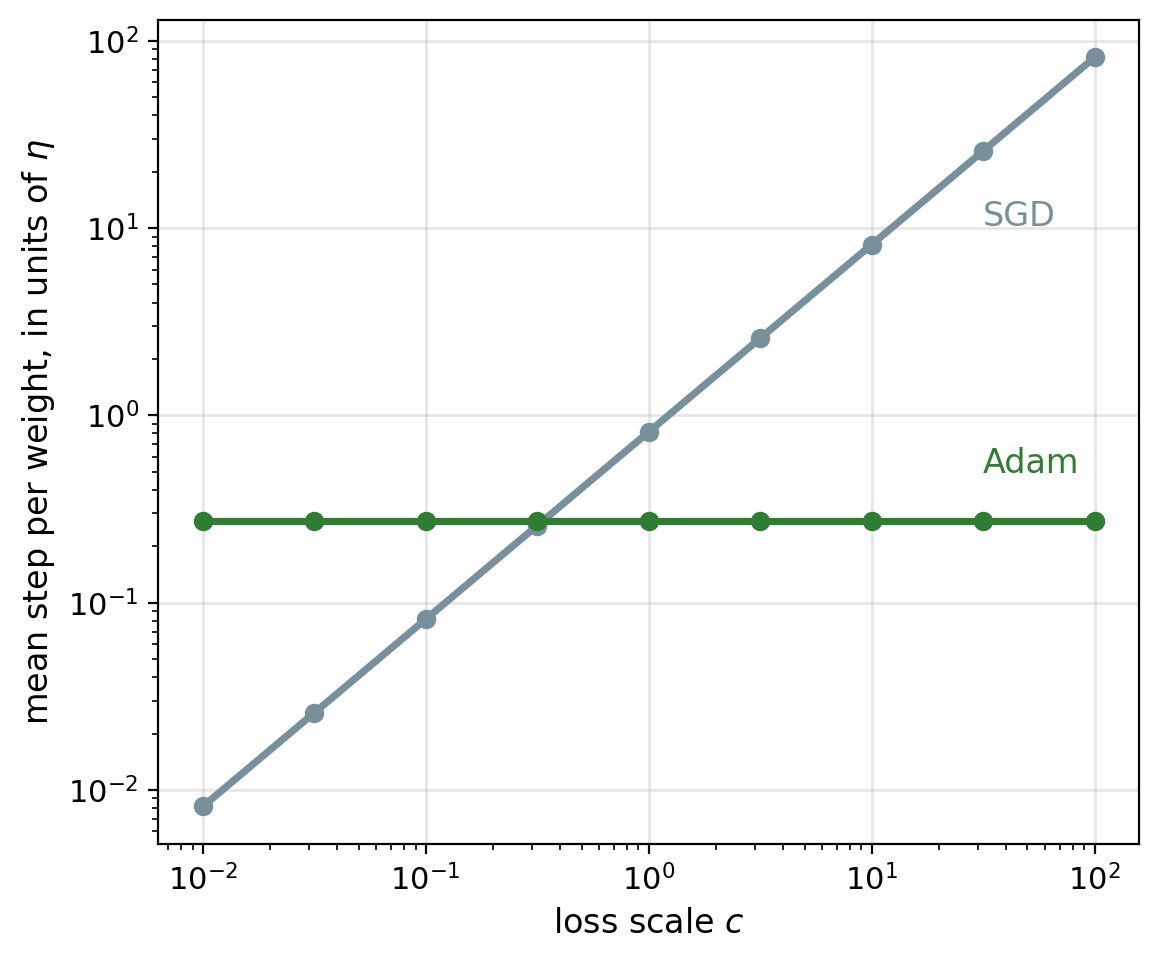
Loss multiplied by \(c\): every gradient multiplied by \(c\)
- SGD: step multiplied by \(c\)
- Adam: \(\hat{m}_t\) and \(\sqrt{\hat{v}_t}\) both multiplied by \(c\), the ratio unchanged
Consequence
- Adam’s step per weight: on the order of \(\eta\), in the units of the weight
- One default, \(\eta = 10^{-3}\), across losses and layers of very different gradient size
- Momentum in Adam: \((1 - \beta_1)\) keeps the average at the gradient’s level, so \(\beta_1\) does not rescale the step
\(\beta_1 = \beta_2 = 0\): the step \(\eta\, \operatorname{sign}(\mathbf{g})\), SignSGD, every weight moved by \(\eta\)
Fitting the Training Set Faster Does Not Lower the Validation Loss
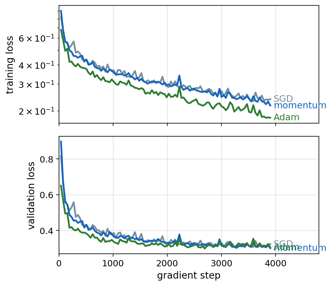
Same network, data, and batch order, one \(\eta\) per optimizer, not tuned
- SGD \(\eta = 0.1\)
- Momentum \(0.9\), \(\eta = 0.01\)
- Adam, \(\eta = 10^{-3}\)
Training loss at the end, two seeds
- Adam: \(0.18\) and \(0.19\)
- Momentum: \(0.23\) and \(0.24\)
- SGD: \(0.24\) and \(0.24\)
Validation loss at the end: within the seed-to-seed spread
- Adam: \(0.305\) and \(0.308\)
- Momentum: \(0.301\) and \(0.311\)
- SGD: \(0.324\) and \(0.306\)
SGD: L2 Penalty Shrinks Every Weight by the Same Factor
L2 penalty \(\tfrac{\lambda}{2}\|\mathbf{w}\|^2\) added to the loss, SGD step

\[\mathbf{w} \leftarrow \mathbf{w} - \eta\,(\mathbf{g} + \lambda \mathbf{w}) = (1 - \eta\lambda)\,\mathbf{w} - \eta\,\mathbf{g}\]
- \(\mathbf{g}\): gradient of the unpenalized loss
- Every weight \(\times (1 - \eta\lambda)\), then the gradient step
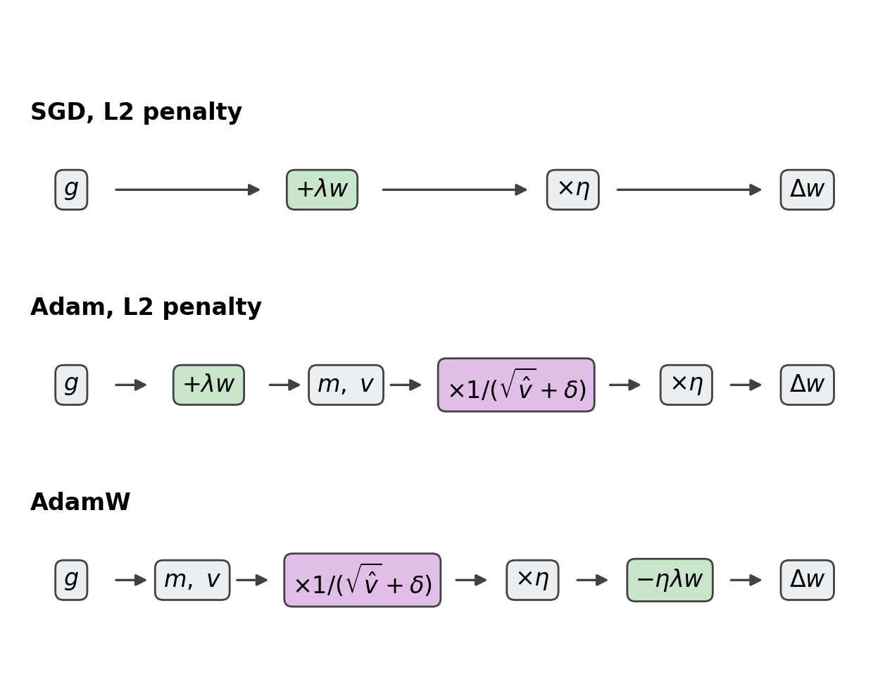
Weight decay: every weight \(\times (1 - \eta\lambda)\) each step, applied outside the loss
- For SGD, the same update as the L2 penalty
SGD(weight_decay=λ): the same update
Adam, for each weight

\[\mathbf{m}_t = \beta_1 \mathbf{m}_{t-1} + (1 - \beta_1)\,\mathbf{g}_t\]
\[\mathbf{v}_t = \beta_2 \mathbf{v}_{t-1} + (1 - \beta_2)\,\mathbf{g}_t^2\]
\[\mathbf{w} \leftarrow \mathbf{w} - \eta\, \frac{\hat{\mathbf{m}}_t}{\sqrt{\hat{\mathbf{v}}_t} + \delta}\]
- \(\hat{\mathbf{m}}_t\), \(\hat{\mathbf{v}}_t\): bias-corrected
- \(\sqrt{\hat{\mathbf{v}}_t}\): the RMS of the weight’s recent gradients
- Step per weight: its filtered gradient divided by that RMS
An L2 Penalty in Adam Decays Weights With Large Gradients Less
Adam with an L2 penalty: \(\lambda \mathbf{w}\) inside \(\mathbf{g}_t\)
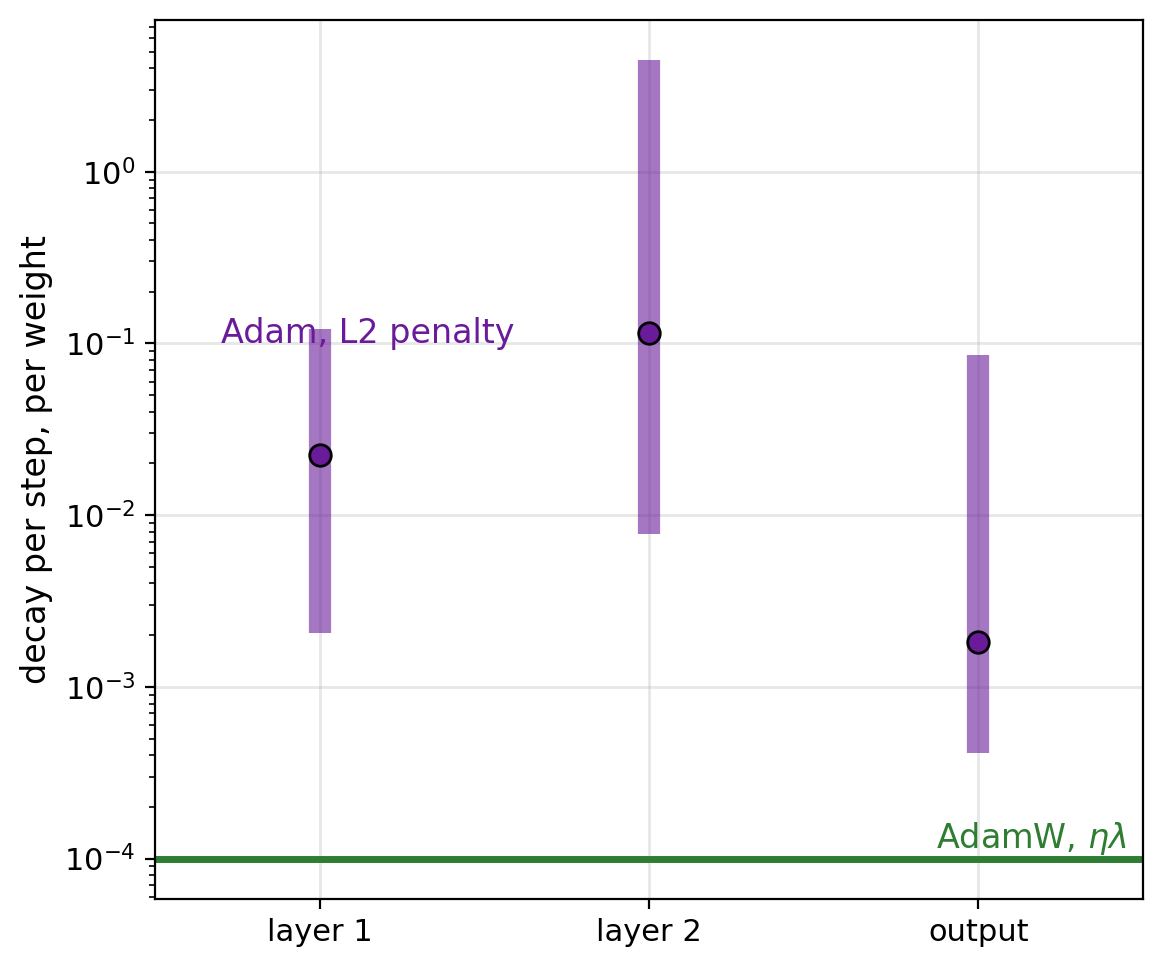
\[\text{decay rate per step} \approx \frac{\eta\lambda}{\sqrt{\hat{v}} + \delta}\]
- Large gradient RMS: slow decay
- Small gradient RMS: fast decay
Gradient RMS \(\sqrt{\hat{v}}\), FashionMNIST, Adam, first layer, end of training
- \(10\)th percentile: \(8.2 \times 10^{-6}\)
- \(90\)th percentile: \(4.8 \times 10^{-4}\)
- First-layer decay rates: a spread of \(59\times\)
AdamW Shrinks Every Weight by the Same Factor
Decoupled weight decay (Loshchilov and Hutter 2019): decay outside the running averages
\[\mathbf{w} \leftarrow (1 - \eta\lambda)\, \mathbf{w} - \eta\, \frac{\hat{\mathbf{m}}_t}{\sqrt{\hat{\mathbf{v}}_t} + \delta}\]
- Shrink factor per step: \(1 - \eta\lambda\), as in SGD
weight_decay in PyTorch
Adam: L2 penalty, inside \(\mathbf{g}_t\), default \(0\)AdamW: decoupled, default \(0.01\)
params = list(model.parameters())
decay = [p for p in params if p.ndim > 1]
other = [p for p in params if p.ndim == 1]
opt = torch.optim.AdamW([
    {'params': decay, 'weight_decay': 0.1},
    {'params': other, 'weight_decay': 0.0},
], lr=1e-3)- Weight matrices decayed; biases and normalization parameters not
AdamW Reaches a Lower Validation Loss Than Adam With an L2 Penalty
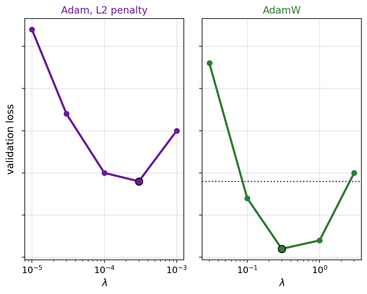
Each form at its best \(\lambda\) (Loshchilov and Hutter 2019)
- AdamW: the lower validation loss
- AdamW: close to its best over a wider range of \(\lambda\)
First-layer weights, per input pixel
- L2 penalty: center weights large, border weights near \(0\)
- AdamW: every weight shrunk alike
Batch Norm: Relative Step \(\propto \eta / \|\mathbf{w}\|^2\)
Batch norm: output independent of the weight scale
- Weights \(\times c\): gradient \(\times 1/c\)
Step relative to the weights: \(\|\Delta \mathbf{w}\| = \eta \|\mathbf{g}\| \propto \eta / \|\mathbf{w}\|\)
\[\frac{\|\Delta \mathbf{w}\|}{\|\mathbf{w}\|} \propto \frac{\eta}{\|\mathbf{w}\|^2}\]
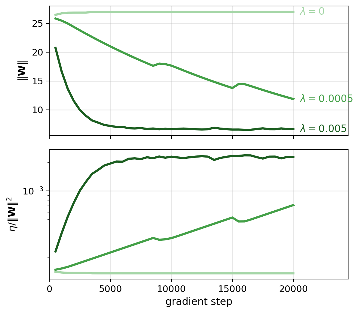
- Effective learning rate: \(\eta / \|\mathbf{w}\|^2\)
- Weight decay: \(\|\mathbf{w}\|\) smaller, effective rate higher
\(\|\mathbf{W}\|\): norm of both hidden weight matrices, SGD \(\eta = 0.1\), \(20{,}000\) steps
- \(\lambda = 0\): \(26.5\) at the start, \(27.0\) at the end
- \(\lambda = 5 \times 10^{-4}\): \(11.8\)
- \(\lambda = 5 \times 10^{-3}\): \(6.6\)
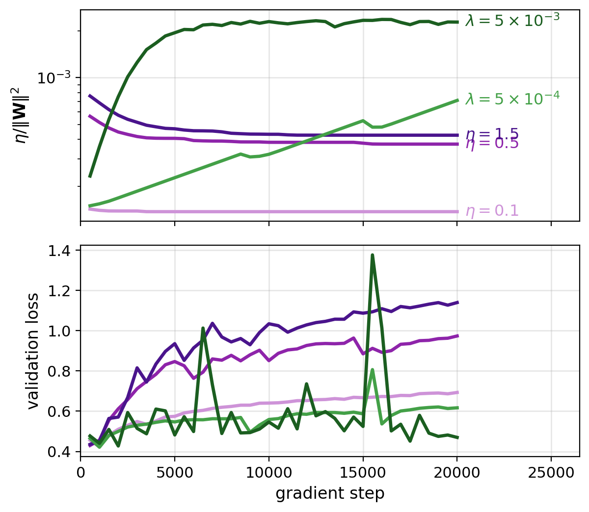
Raising \(\eta\) Does Not Replace Weight Decay Under Batch Norm
Batch-normalized layers: shrinking \(\mathbf{w}\) leaves the output unchanged
Raising \(\eta\) without decay: \(\|\mathbf{w}\|\) grows with it
- \(\eta = 0.1\), \(0.5\), \(1.5\): \(\|\mathbf{W}\|\) at the end \(27.0\), \(36.6\), \(59.3\)
- Effective rate: at most \(4.3 \times 10^{-4}\)
Weight decay \(\lambda = 5 \times 10^{-3}\), \(\eta = 0.1\): effective rate \(2.3 \times 10^{-3}\)
- Validation loss at the end: \(0.69\) with \(\lambda = 0\), \(0.47\) with \(\lambda = 5 \times 10^{-3}\)
- The best \(\eta\) depends on \(\lambda\)
Output layer, no batch norm: weight decay is an L2 penalty
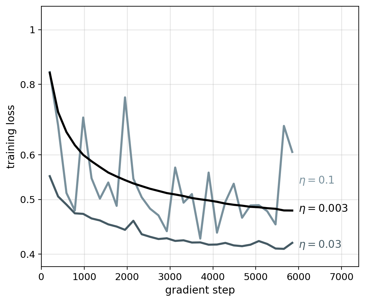
SGD’s Noise Floor Grows With the Learning Rate
Noise floor: the level SGD levels off at with a constant \(\eta\), above the minimum, because minibatch gradients are noisy
\[\mathbb{E}\big[\|\mathbf{w}_t - \mathbf{w}^*\|^2\big] \le (1 - \eta\mu)^t \|\mathbf{w}_0 - \mathbf{w}^*\|^2 + O\Big(\frac{\eta\, \sigma_g^2}{\mu}\Big)\]
- \(\mu\): the smallest curvature; \(\sigma_g^2\): the gradient noise variance
- First term: decays as \((1 - \eta\mu)^t\), faster for larger \(\eta\)
- Second term: the floor, proportional to \(\eta\)
- As in LMS: misadjustment proportional to the step size
Logistic regression, FashionMNIST, SGD, training loss after \(15\) epochs
- \(\eta = 0.1\): \(0.54\), noisy
- \(\eta = 0.03\): \(0.42\)
- \(\eta = 0.003\): \(0.48\), still falling
Each Drop in the Learning Rate Lowers the Noise Floor
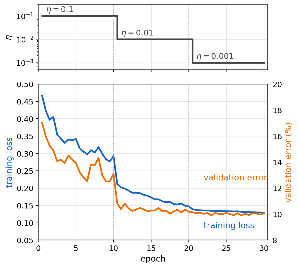
Learning-rate schedule: \(\eta_t\), the learning rate as a function of the step
Noise floor: proportional to the current \(\eta\)
- Noise in each step: proportional to \(\eta\)
- After a drop: a lower floor
- After a drop, the loss starts from the level reached at the larger \(\eta\)
Step decay, \(\eta \times 0.1\) at epochs \(10\) and \(20\), SGD with momentum
- Training loss, last \(2\) epochs before each drop and at the end: \(0.288\), \(0.151\), \(0.130\)
- Validation error: \(12.8\%\), \(10.2\%\), \(10.0\%\)
sched = torch.optim.lr_scheduler.MultiStepLR(
    opt, milestones=[10, 20], gamma=0.1)
for epoch in range(30):
    for x, y in batches:
        loss = loss_fn(model(x), y)
        opt.zero_grad()
        loss.backward()
        opt.step()
sched.step()sched.step()once per epoch: milestones count epochs
Schedules With a Similar Final Learning Rate End at a Similar Loss
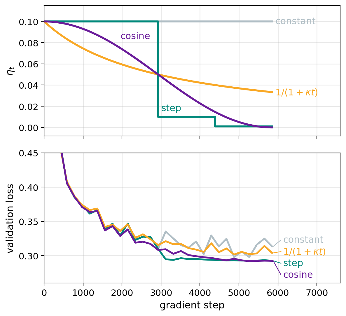
Noise floor at the end: proportional to the final \(\eta\)
Validation loss after \(15\) epochs (\(T\) steps), MLP, \(\eta_0 = 0.1\)
- Constant, final \(\eta = 0.1\): \(0.314\)
- \(1/(1 + \kappa t)\), \(\kappa = 2/T\), final \(\eta = 0.033\): \(0.304\)
- Step decay, \(\times 0.1\) at \(50\%\) and \(75\%\), final \(\eta = 0.001\): \(0.293\)
- Cosine, final \(\eta = 0\): \(0.293\)
Cosine: \(\eta_t = \tfrac{\eta_0}{2}\big(1 + \cos(\pi t / T)\big)\)
\(\eta_0/(1 + \kappa t)\): decays as \(1/t\), equal to \(\eta_0\) at \(t = 0\)
In PyTorch
MultiStepLR(opt, milestones, gamma)LambdaLR(opt, lambda t: 1 / (1 + kappa * t))CosineAnnealingLR(opt, T_max)
Restarted Annealing Schedules Reach a Lower Loss Each Cycle
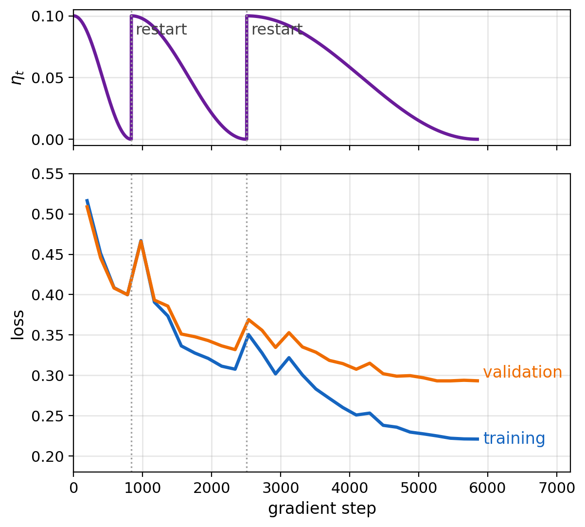
Noise floor: proportional to the current \(\eta\), rising or falling
- Raising \(\eta\): the loss rises
- Next decay: the loss ends below its value before the rise
Warm restarts (SGDR): \(\eta\) reset to \(\eta_0\), then a new cosine decay
Measured, MLP, training loss at each restart
- First: \(0.400\) before, \(0.467\) after
- Second: \(0.308\) before, \(0.350\) after
- End of the last decay: \(0.221\)
Schedules that raise \(\eta\)
- Warm restarts: a low-loss network at the end of every cycle
- One-cycle: a rise to a peak \(\eta\) above a decay-only schedule’s start, then one decay
- Warmup, stable, decay: constant \(\eta\), then a short decay started from any checkpoint
Warmup Reduces Adam’s High-Variance Early Steps
Adam’s step, per weight: \(\eta\, \hat{m}_t / \sqrt{\hat{v}_t}\)
- Step \(1\): \(\hat{m}_1 = g_1\) and \(\hat{v}_1 = g_1^2\), so \(|\hat{m}_1 / \sqrt{\hat{v}_1}| = 1\)
- \(\hat{m}_t\), \(\hat{v}_t\) from few gradients: estimates with high variance
- Every weight moves by \(\eta\), whatever its gradient
- First steps: \(\hat{m}_t\) and \(\hat{v}_t\) average few gradients, the step well above its long-run size
Simulated gradients, a small mean plus unit noise per weight, mean step size in units of \(\eta\)
- Step \(1\): \(1.0\); step \(10\): \(0.28\); from step \(50\) on: \(0.2\)
Warmup: \(\eta_t = \eta \cdot \min(1,\ t / t_w)\), over the first \(t_w\) steps
- Small steps while \(\hat{m}_t\) and \(\hat{v}_t\) average few gradients
- Full \(\eta\) once they average many
warm = torch.optim.lr_scheduler.LinearLR(
    opt, start_factor=0.01, total_iters=100)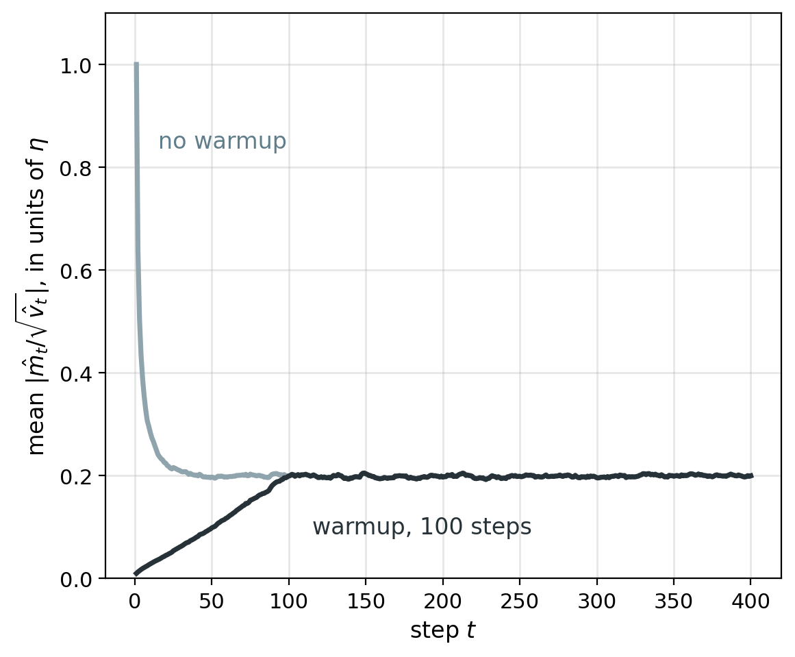
Clipping by Norm Lowers the Learning Rate on Steps With Large Gradients
Clipping by norm, threshold \(c\)
\[\mathbf{g} \leftarrow \mathbf{g} \cdot \min\Big(1,\ \frac{c}{\|\mathbf{g}\|}\Big)\]
- Clipped \(\mathbf{g}\): \(\mathbf{g}\) scaled by \(c/\|\mathbf{g}\|\), the same as a smaller \(\eta\) for that step
- SGD step length: \(\min(\eta\|\mathbf{g}\|,\ \eta c)\)
Clipping by value: each component clipped to \([-c, c]\)
- Components with \(|g_i| > c\) set to \(\pm c\), others unchanged
- Clipped \(\mathbf{g}\) no longer parallel to \(\mathbf{g}\)
- \(c\) below every \(|g_i|\): \(c \cdot \operatorname{sign}(\mathbf{g})\), the SignSGD step
loss.backward()
torch.nn.utils.clip_grad_norm_(
    model.parameters(), max_norm=1.0)
opt.step()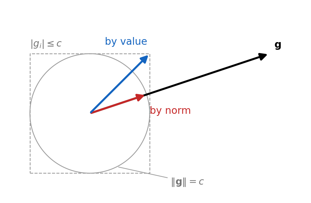
Gradient Clipping Prevents Diverging Weight Updates
Gradient descent on a quadratic with curvature \(h\): stable for \(\eta h < 2\)
- \(\eta h > 2\): the error multiplies by \(|1 - \eta h| > 1\) each step
Deep network: the gradient is a product of the layers’ weights and slopes
- An overshoot that enlarges the weights enlarges the next gradient
Clipping: next step length at most \(\eta c\), whatever the gradient
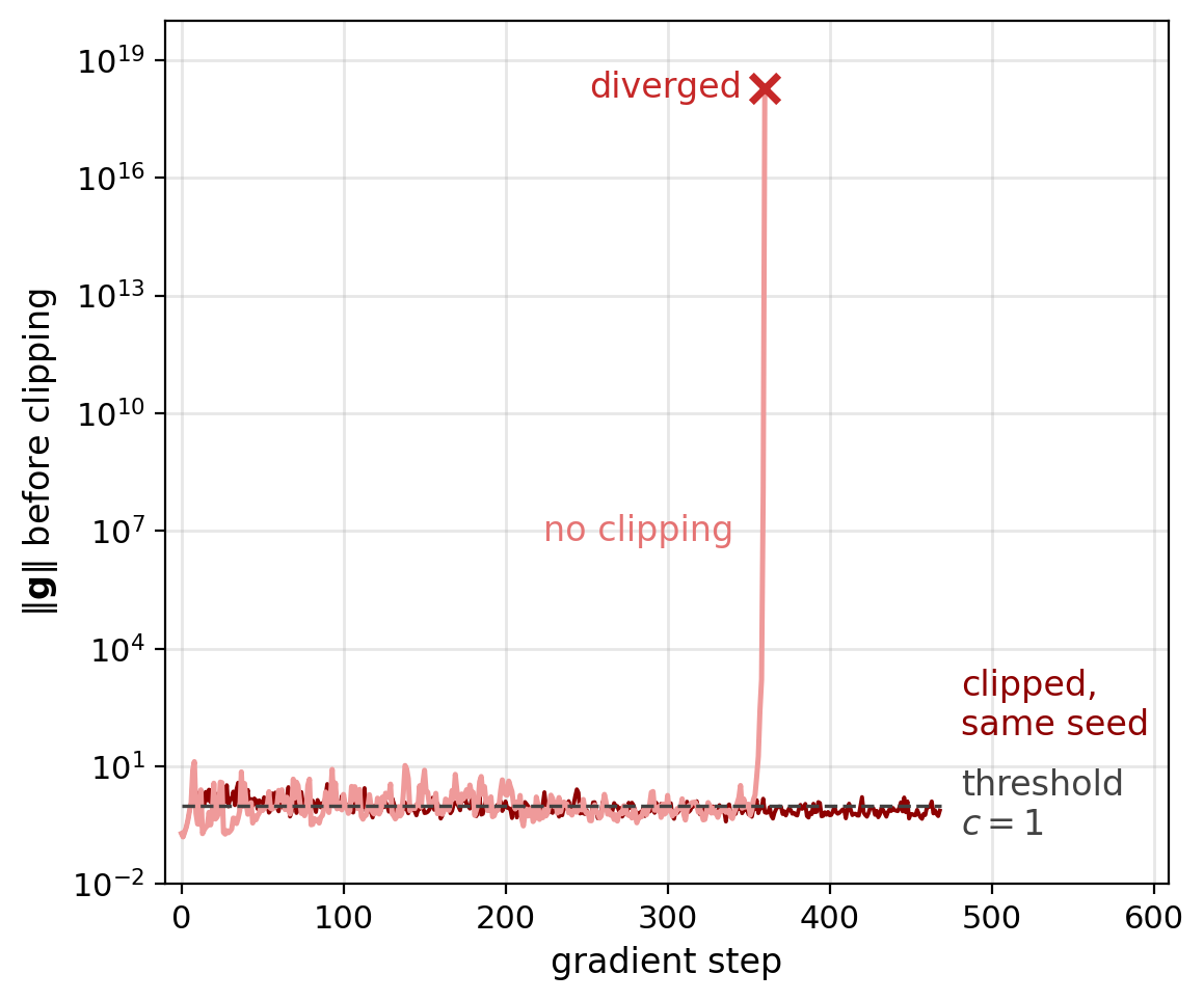
Four hidden layers of \(256\) units, SGD \(\eta = 1.0\), one epoch
- Median \(\|\mathbf{g}\|\), first \(100\) steps: \(0.75\), so most steps are not clipped
- Diverging seed, \(\|\mathbf{g}\|\) on four consecutive steps before overflow: \(5\), \(18\), \(263\), \(1{,}633\)
- No clipping: \(1\) of \(3\) seeds diverged
- No clipping, test accuracy of the other two: \(74\%\), \(65\%\)
- Clipping at \(c = 1\): no seed diverged, test accuracy \(82\%\) for each
Learning-Rate Schedules Add Heuristic Hyperparameters
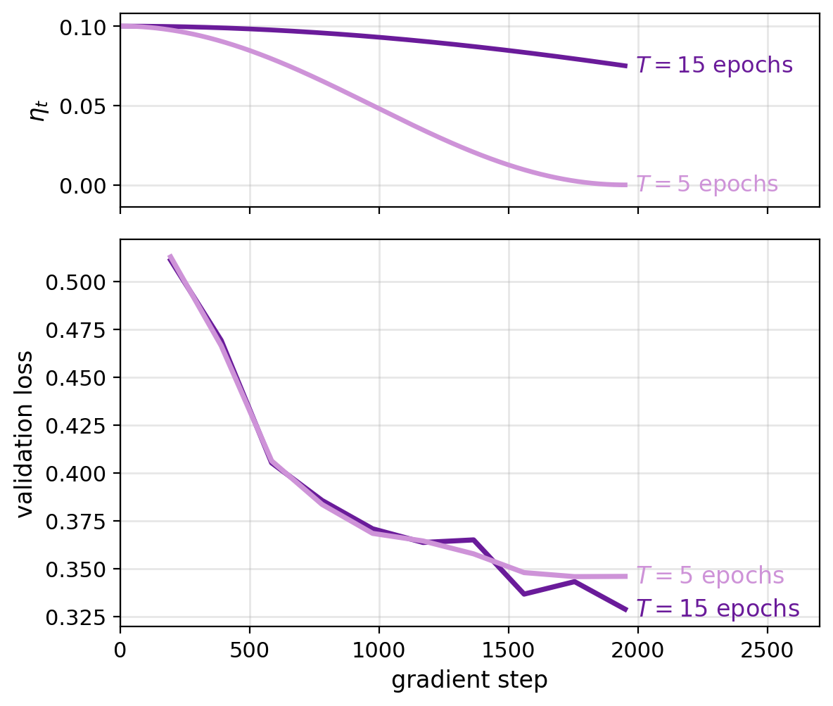
Cosine and step decay: \(T\) set before the first step
- \(\eta\) small only near \(T\)
Cosine from \(0.1\), validation loss at epoch \(5\)
- \(T = 15\) epochs: \(0.329\), \(\eta\) still \(0.075\)
- \(T = 5\) epochs: \(0.346\), \(\eta\) already \(0\)
- Different networks at the same epoch: \(T\) is a setting
\(T\) too short: \(\eta\) near \(0\) while the loss is still falling
Hyperparameters of a schedule, chosen by rule of thumb before training
- Shape: step, \(1/(1 + \kappa t)\), cosine, restarts
- Length \(T\), milestones, decay factor, warmup steps
Training length
- Early stopping: chosen during training, from the validation curve
- A decaying schedule: chosen before training
Choosing a Hyperparameter Costs One Training Run per Value
Hyperparameter \(h\): a setting that training does not adjust
- \(\lambda\), dropout \(p\), label smoothing \(\varepsilon\), patience, \(\eta\), its schedule, \(c\)
Two nested problems
\[h^* = \arg\min_h\ \mathcal{L}_{\text{val}}\big(\mathbf{w}^*(h)\big), \qquad \mathbf{w}^*(h) = \arg\min_{\mathbf{w}}\ \mathcal{L}_{\text{train}}(\mathbf{w};\, h)\]
- Inner problem: a full training run for each \(h\)
- Outer objective: known only at the values of \(h\) trained
- No gradient with respect to \(h\) from one run: the search compares runs
Outer objective on validation data
- Training loss is lowest at \(\lambda = 0\): a regularizer raises it to lower validation loss
Most Grid Runs Vary Hyperparameters That Barely Change the Loss
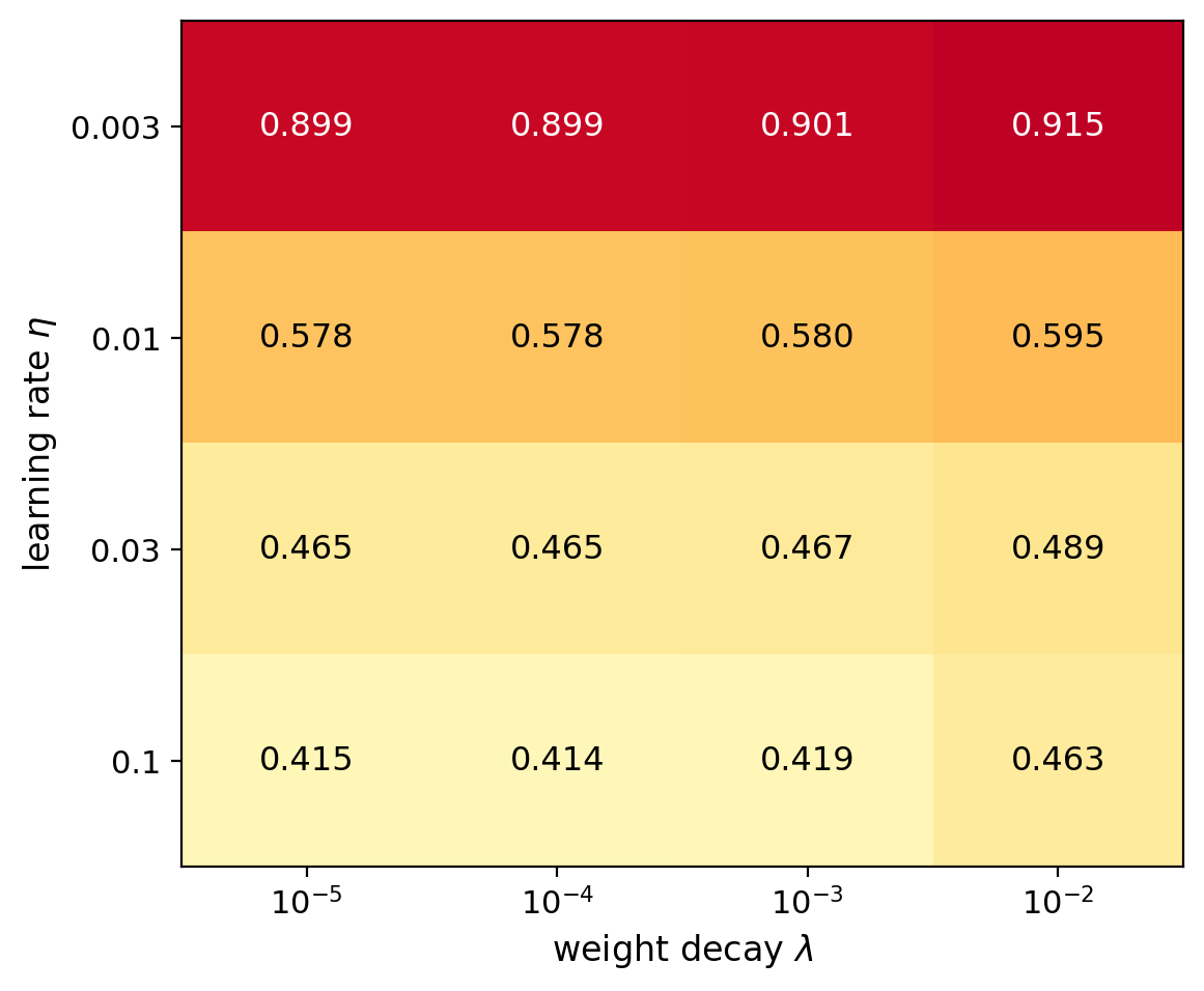
Grid search: \(k\) values of each of \(d\) hyperparameters, every combination, \(k^d\) runs
Measured, \(4 \times 4\) grid, validation loss after \(10\) epochs
- At each \(\lambda \le 10^{-3}\), across \(\eta\): from about \(0.4\) to \(0.9\)
- At each \(\eta\), across \(\lambda \le 10^{-3}\): under \(0.005\)
- \(16\) runs, \(4\) values of \(\eta\)
Effective dimension: the loss depends on few of the hyperparameters
- Runs spent varying the others measure almost nothing
Random Settings Give Every Hyperparameter a New Value in Every Run
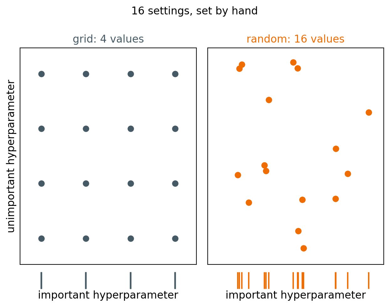
Random search (Bergstra and Bengio 2012): each setting drawn at random, independently per hyperparameter
\(N\) runs
- Grid of \(d\) hyperparameters: \(N^{1/d}\) values of each
- Random: \(N\) values of each, the important ones included
Measured, \(16\) runs each
- Grid: \(4\) values of \(\eta\)
- Random: \(16\) values of \(\eta\)
Useful Learning Rates Span Several Orders of Magnitude
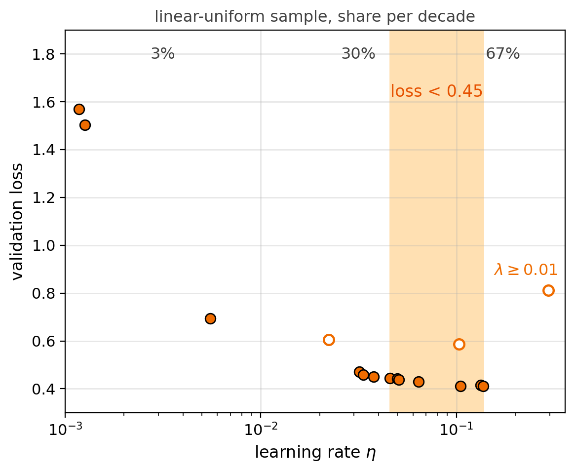
Range searched: \(\eta\) from \(0.001\) to \(0.3\), \(2.5\) orders of magnitude
- Validation loss below \(0.45\): \(\eta\) from \(0.046\) to \(0.137\)
- Below \(\eta = 0.01\): every run above \(0.65\)
Linear-uniform sampling on \([0.001, 0.3]\)
- \(90\%\) of samples above \(0.03\)
- \(3\%\) between \(0.001\) and \(0.01\)
Log-uniform sampling: \(\log \eta\) uniform
- The same share of samples per factor of \(10\)
- For \(\eta\) and \(\lambda\), whose effects scale with their size
Stopping Poor Settings Early Saves Most of the Search Cost
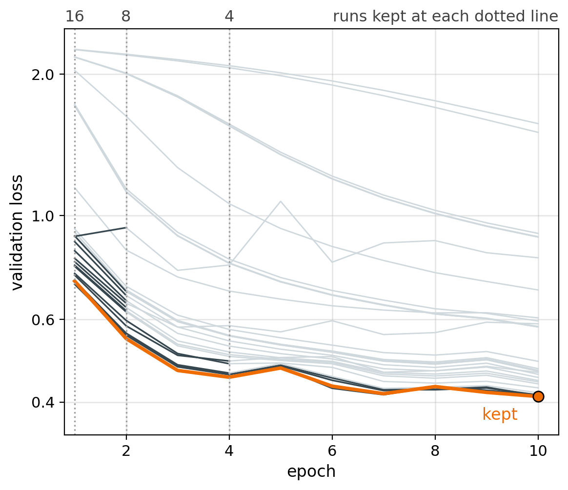
Most settings are poor: of \(32\), the poor ones are already poor after \(1\) epoch
Rank agreement with the final validation loss, \(32\) runs (Spearman)
- After \(1\) epoch: \(0.93\)
- After \(2\) epochs: \(0.95\)
- After \(4\) epochs: \(0.98\)
Successive halving (Jamieson and Talwalkar 2016): every setting trained briefly, the better half continued, repeated
- \(32\) settings, halved after epochs \(1\), \(2\), \(4\)
- Cost: \(88\) epochs, against \(320\) to train every setting fully
Its assumption: early rank predicts final rank
- Fails for settings that start slowly and finish well, a small \(\eta\) among them
The Seed Can Affect the Loss More Than a Hyperparameter
Seed: the random start and the batch order
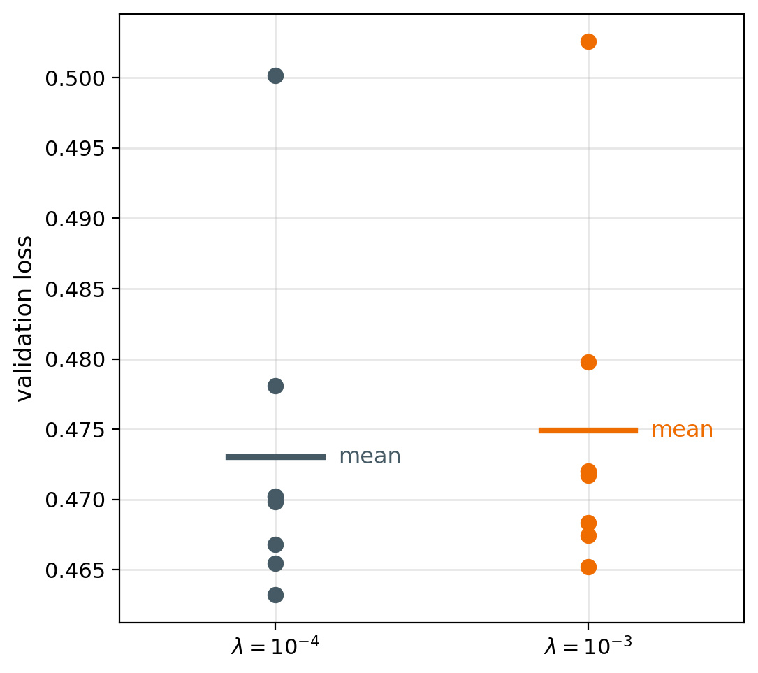
One setting, \(8\) seeds, \(\eta = 0.03\), \(\lambda = 10^{-4}\)
- Validation loss: \(0.463\) to \(0.500\)
- Standard deviation: \(0.012\)
Changing \(\lambda\) to \(10^{-3}\): mean validation loss up by \(0.0019\)
- \(6\times\) smaller than the standard deviation over seeds
- Two runs with different seeds: the order of their losses is random
Same-Seed Comparisons Isolate a Hyperparameter’s Effect
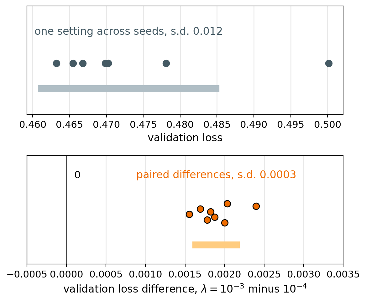
Paired comparison: both settings run with the same seeds, the difference taken seed by seed
- \(L_A\), \(L_B\): validation losses of settings \(A\) and \(B\) on the same seed
\[\mathrm{Var}(L_B - L_A) = \mathrm{Var}(L_A) + \mathrm{Var}(L_B) - 2\,\mathrm{Cov}(L_A, L_B)\]
- Same seed: same start and same batch order
- Nearby settings on the same seed: \(L_A\) and \(L_B\) move together, a large covariance
Measured, the same \(8\) seeds, \(\lambda = 10^{-3}\) minus \(\lambda = 10^{-4}\)
- Differences: \(0.0016\) to \(0.0024\), all positive
- Standard deviation of the difference: \(0.0003\), against \(0.012\) for either setting alone
- Settings far apart (very different \(\eta\)): smaller covariance, less removed
The Lowest Validation Loss Underestimates the True Loss
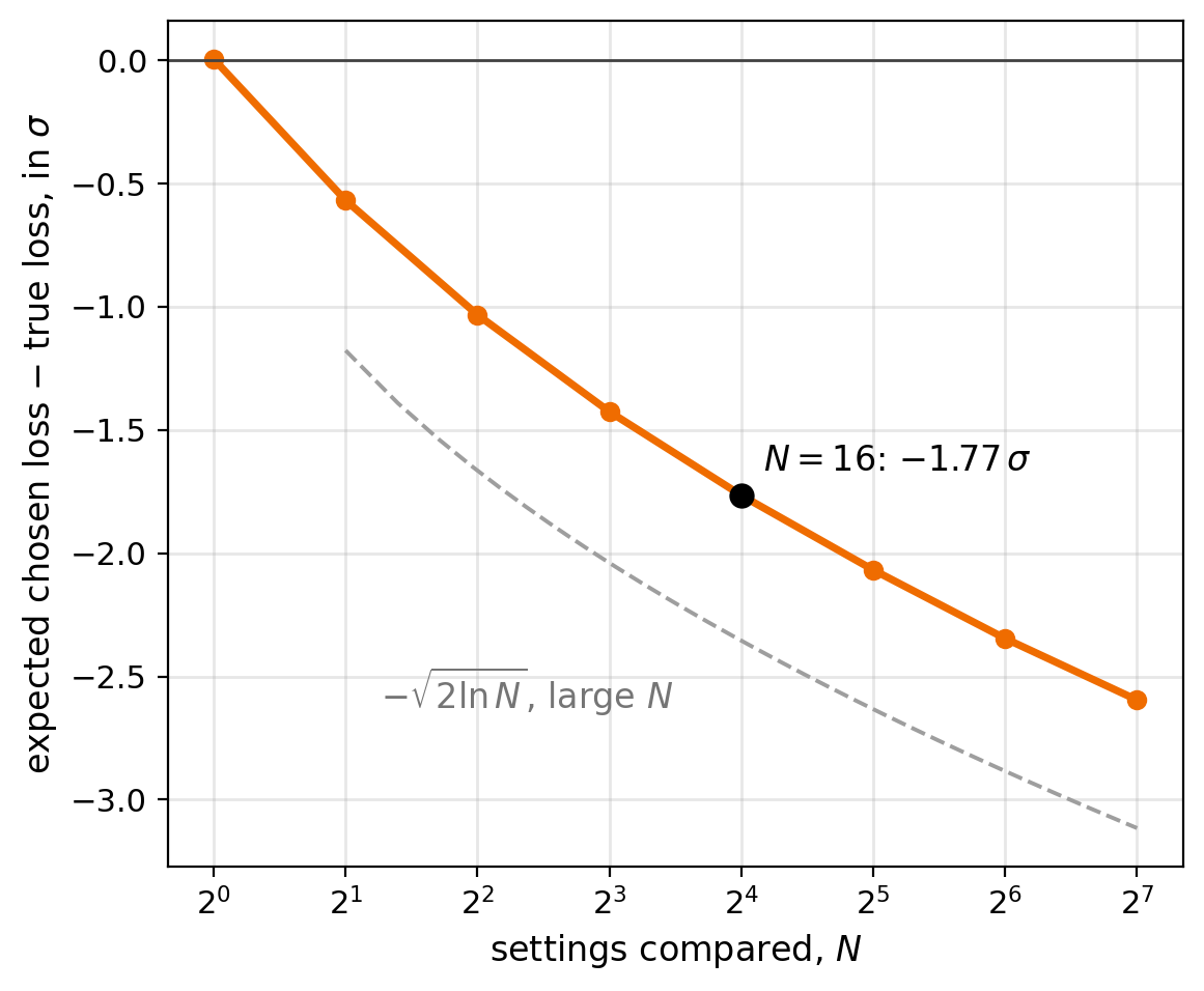
Choosing the minimum of \(N\) noisy validation losses: the chosen value is low partly by chance
- \(N\) settings with the same true loss, noise of standard deviation \(\sigma\)
- Expected lowest value: \(1.77\,\sigma\) below the true loss for \(N = 16\)
- Approaches \(\sqrt{2 \ln N}\,\sigma\) for large \(N\): \(2.35\,\sigma\) at \(N = 16\)
Consequence: the chosen setting’s validation loss overstates its quality
- The test set, used once on the chosen setting, carries no selection
Fixed Budgets Limit Tuning Resolution
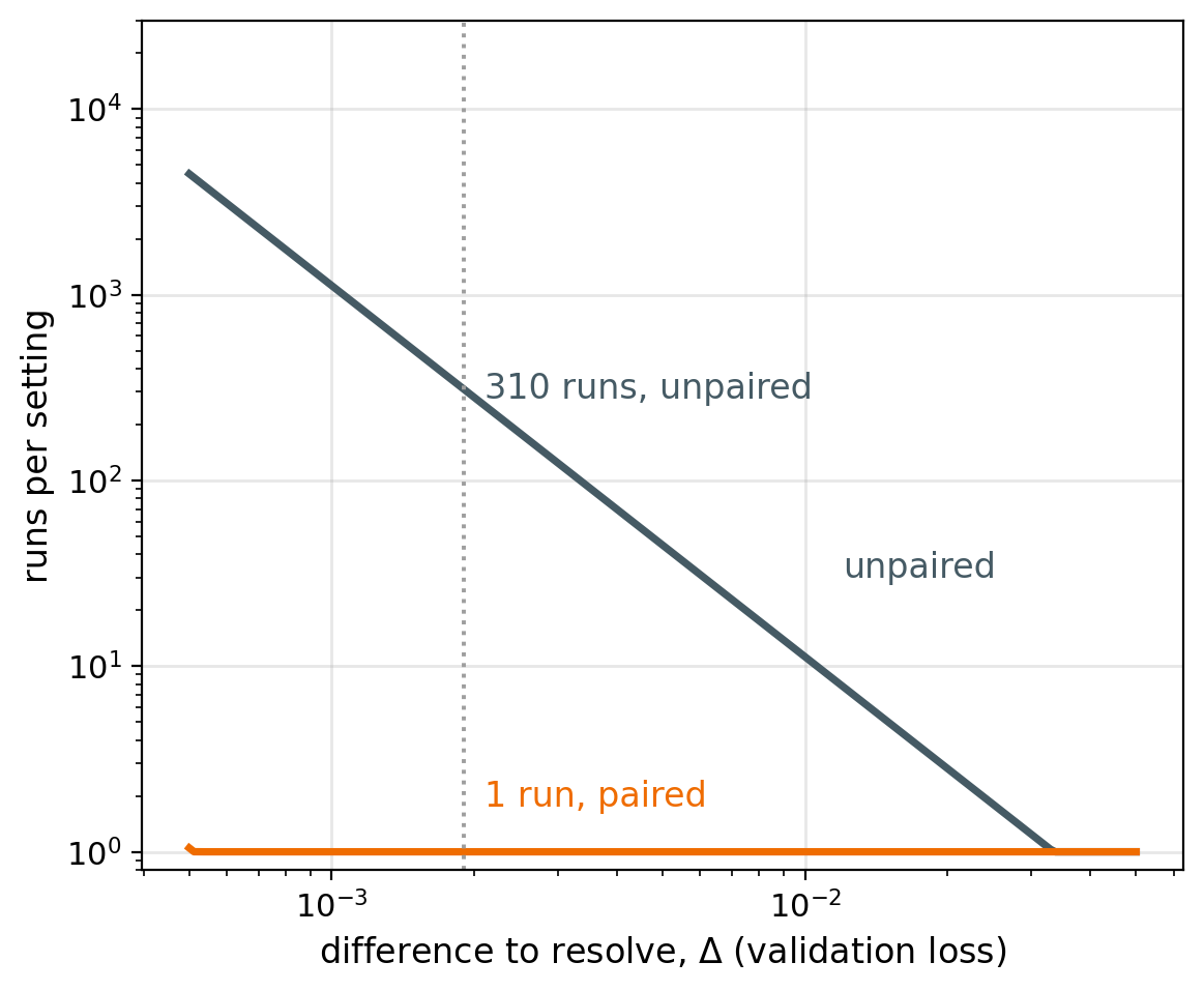
Runs to resolve a difference \(\Delta\) at two standard errors
- Unpaired, seed spread \(\sigma\): about \(2\,(2\sigma/\Delta)^2\) runs per setting
- Paired, spread of the difference \(\sigma_d\): about \((2\sigma_d/\Delta)^2\)
Measured spreads: \(\sigma = 0.012\), \(\sigma_d = 0.0003\)
- \(\Delta = 0.0019\), the \(\lambda\) change: about \(310\) unpaired runs per setting, \(1\) paired
Every hyperparameter searched multiplies the settings, every small effect multiplies the seeds
- Hyperparameters left unsearched: set by defaults and rules of thumb