Convolutional Networks
EE 541 - Unit 8A
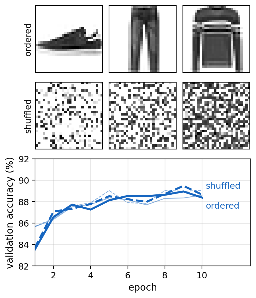
Dense Networks Are Sensitive to Small Shifts
Column \((i, j)\) of \(\mathbf{W}\) multiplies pixel \((i, j)\) and no other
- A trained unit’s weights form a template of the items it responds to, at fixed pixels
- The same edge at two positions is multiplied by two different sets of weights
FashionMNIST is centered: each part of an item at nearly the same pixels in every image
- Shifted item: each part at pixels where the training images had other parts
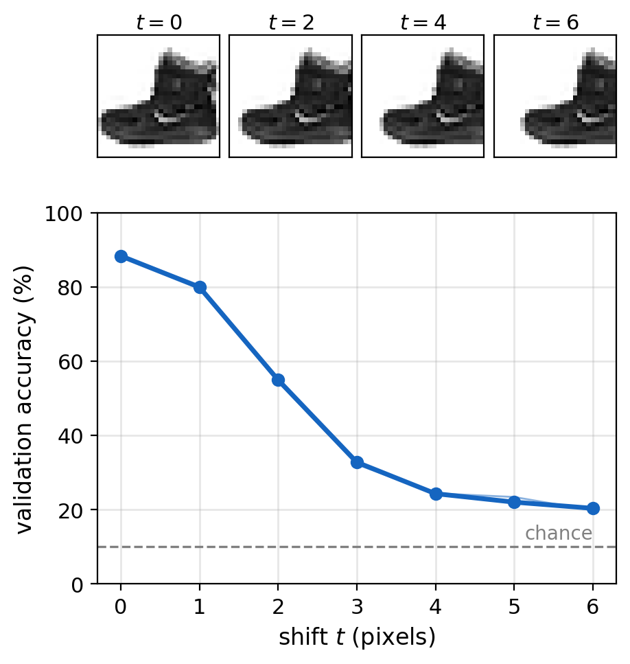
Validation images shifted right by \(t\) pixels, the network trained on centered images
- \(t = 0\): 88.4\(\%\)
- \(t = 2\): 55.0\(\%\)
- \(t = 4\): 24.3\(\%\)
Nearby Pixels Are Strongly Correlated
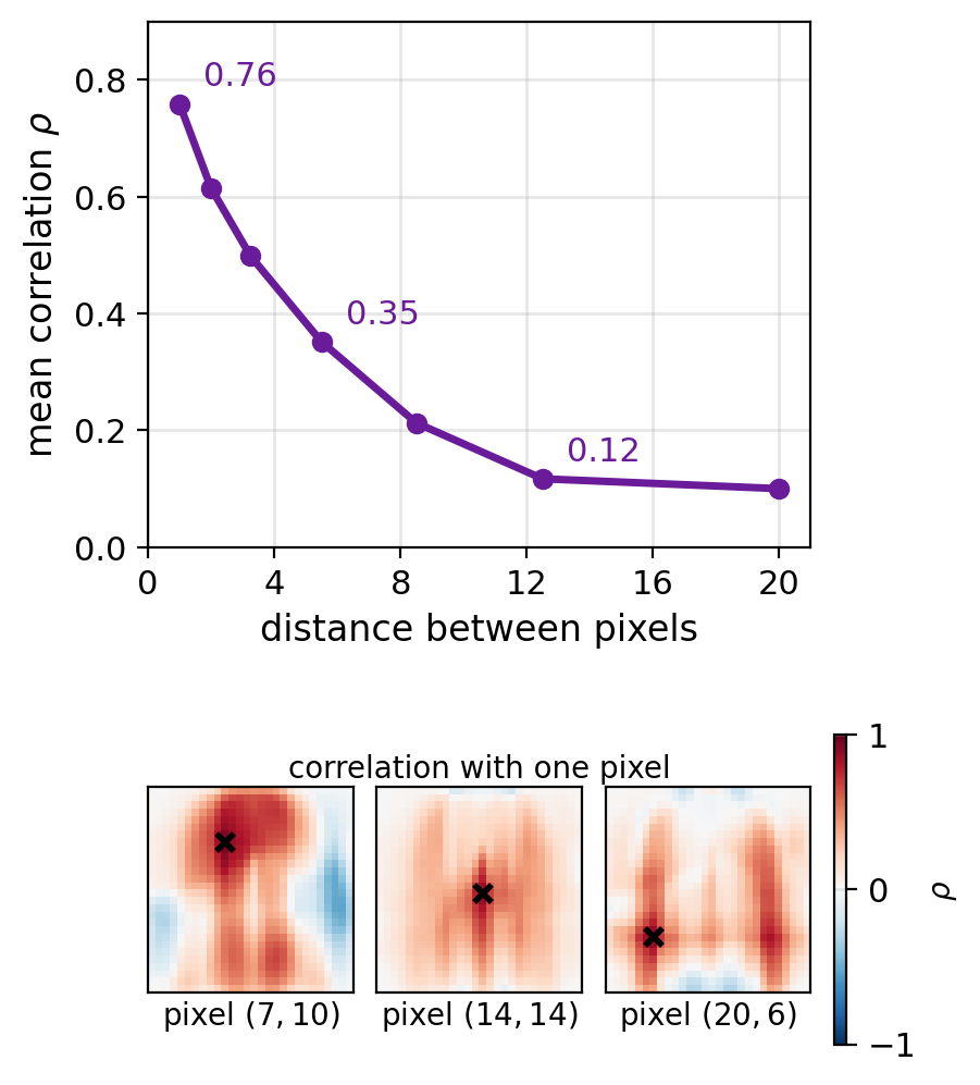
Correlation of two pixels’ intensities over \(20{,}000\) training images \[\rho_{(i,j),(i',j')} = \frac{\mathrm{Cov}(X_{ij}, X_{i'j'})}{\sigma_{ij}\, \sigma_{i'j'}}\]
Average over pixel pairs that vary across images, by distance
- \(1\) pixel apart: \(\rho\) = 0.76
- \(4\) to \(7\) pixels apart: \(\rho\) = 0.35
- \(10\) to \(15\) pixels apart: \(\rho\) = 0.12
Local patterns: edges, stripes, and corners are relations between nearby pixels
Patch: a pixel’s strongest correlations are with its immediate neighbors
Distant correlation: one part of an item with another, such as the two legs of a trouser
One Small Detector Locates Its Pattern at Every Position
Detector: a \(3 \times 3\) array of weights
- Response at a position: the inner product of the weights with the \(3 \times 3\) patch there
- Large where the patch has the weights’ pattern of light and dark, as for a hidden unit’s template over the whole image
Feature map: the response at every position, itself an image
Two detectors
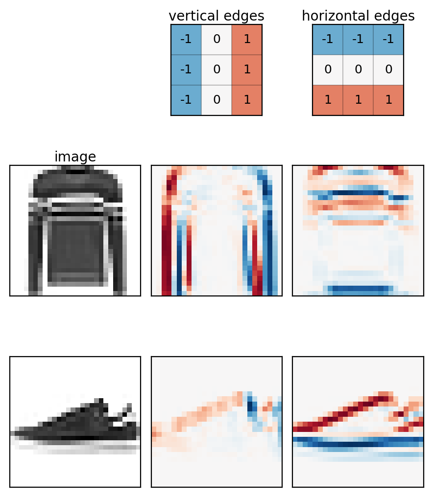
- Right column minus left column: vertical edges
- Bottom row minus top row: horizontal edges
Convolution: computing the response at every position
- Kernel: the detector’s weights
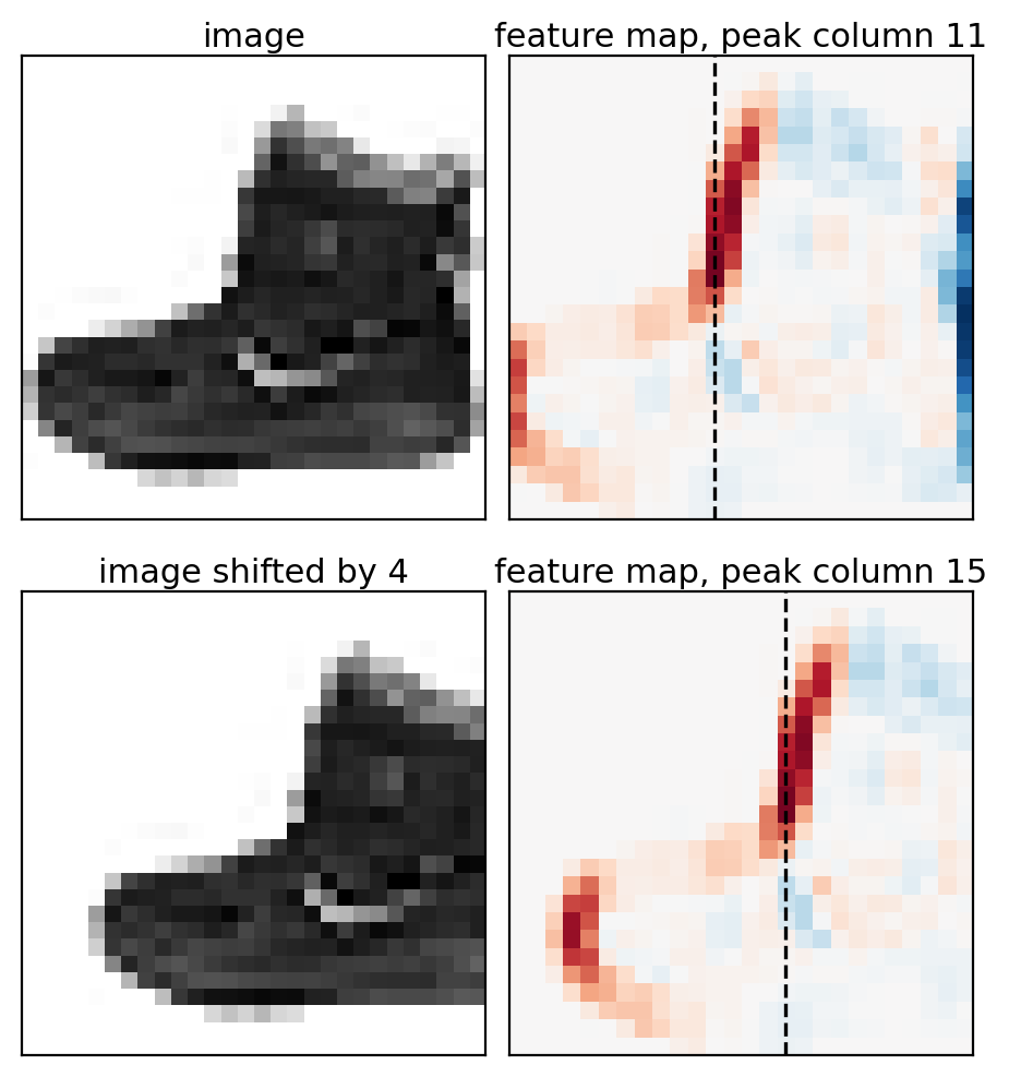
Feature Maps Shift With the Input
Same kernel at every position: an edge gives the same response wherever it is
Vertical-edge kernel, ankle boot shifted right by \(4\) pixels
- Map shifted right by \(4\), the same values
- Except at the borders, where content enters or leaves the frame
Convolutional Networks Are More Accurate With Fewer Parameters
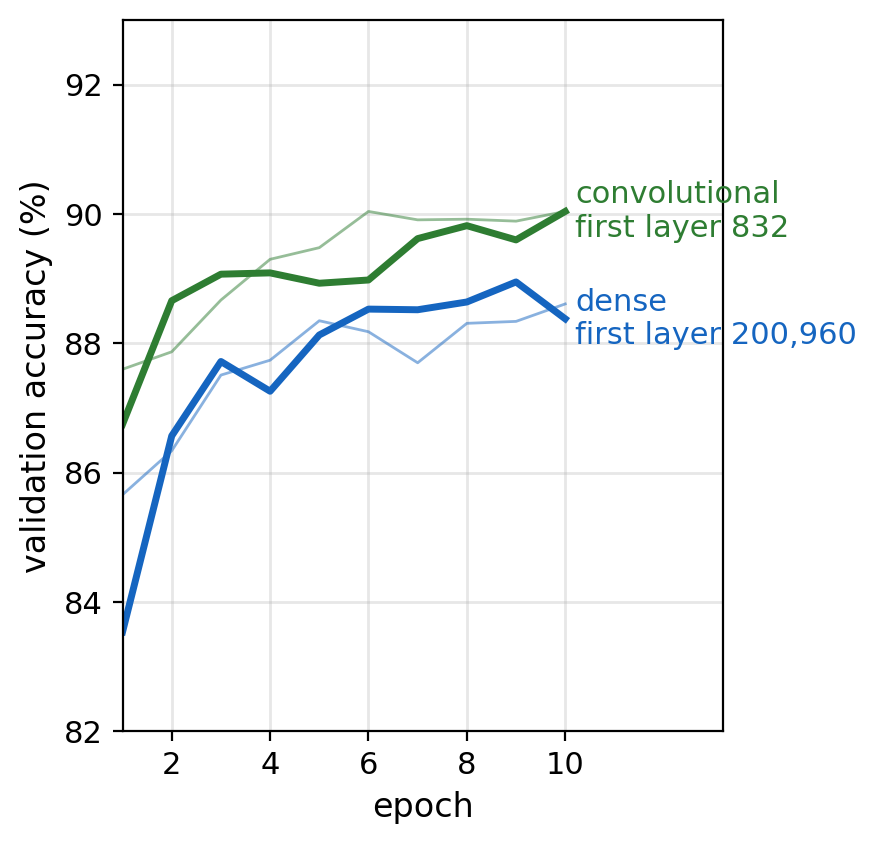
Convolutional network: one layer of \(32\) learned \(5 \times 5\) kernels, ReLU, a dense output layer
- First layer: \(832\) parameters
- \(185{,}162\) parameters in all
Dense network: two hidden layers of \(256\) ReLU units, a dense output layer
- First layer: \(256 \times 785 = 200{,}960\) parameters
- \(269{,}322\) parameters in all
Training: the same optimizer and batch size, \(10\) epochs
- Validation accuracy: 90.0\(\%\) convolutional, 88.4\(\%\) dense
First layer: \(200{,}960 / 832 \approx 242\)
Dense Output Layers Are Not Shift Invariant
Shift invariance: class scores unchanged by a shift
Dense output layer: one weight per feature-map value and class
- \(18{,}432 \times 10 + 10 = 184{,}330\) parameters
- 99.6\(\%\) of the network’s
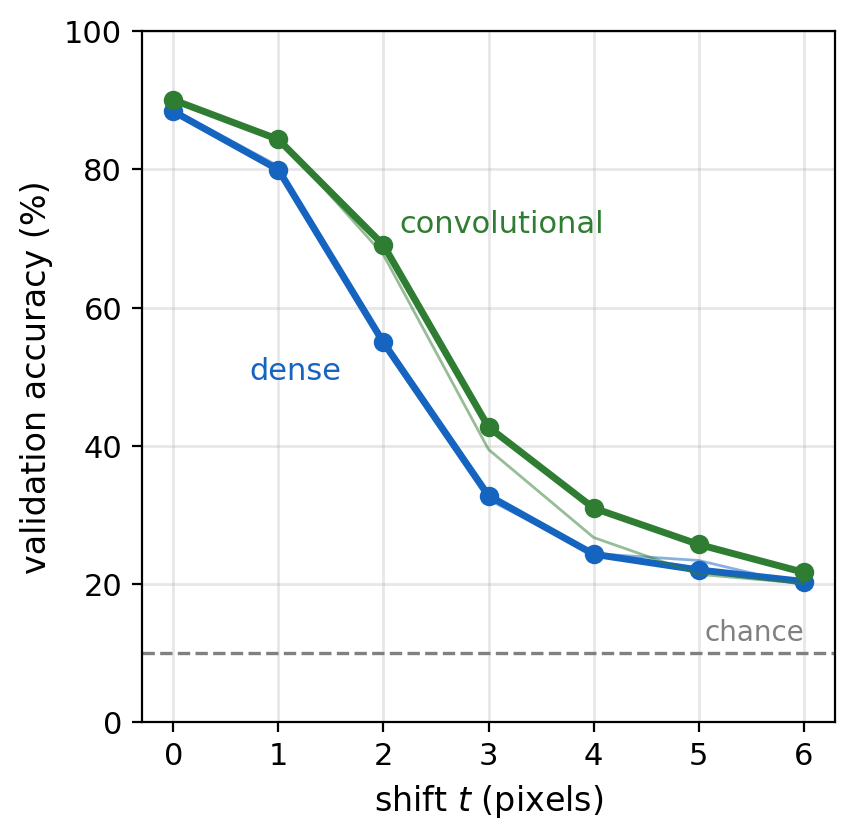
Validation images shifted right by \(t\) pixels
- \(t = 2\): convolutional 69.1\(\%\), dense 55.0\(\%\)
- \(t = 6\): convolutional 21.7\(\%\), dense 20.4\(\%\)
Convolutional Networks Can Classify Thousands of Objects
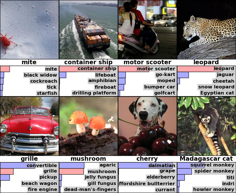
Classification: the true class and the five most probable of \(1{,}000\), for each test image A. Krizhevsky, I. Sutskever, G. E. Hinton, “ImageNet Classification with Deep Convolutional Neural Networks,” NIPS 2012, Fig. 4
Classifiers Can Separate Fine-Grained Classes
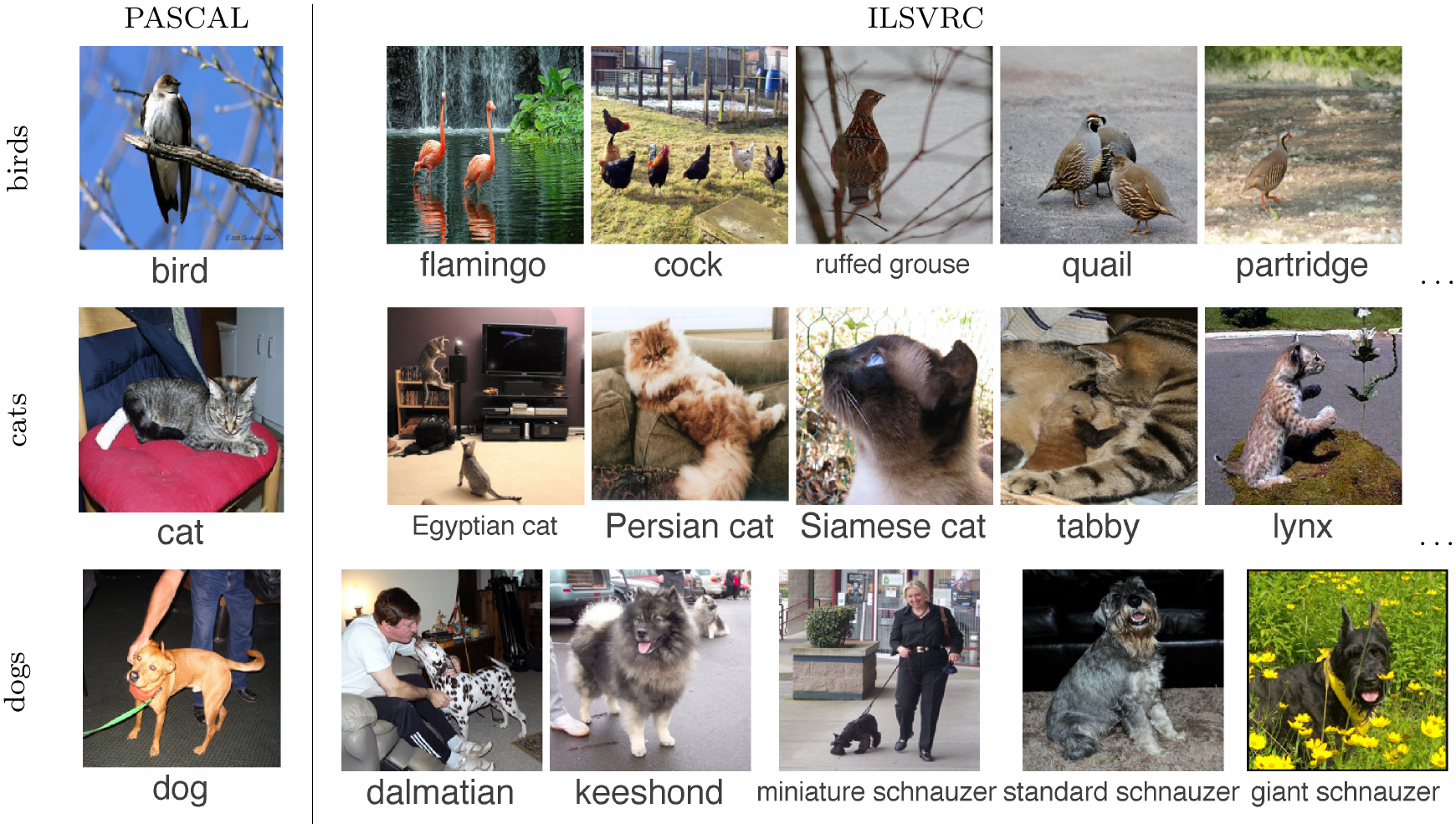
ImageNet: \(1.2\) million photographs in \(1{,}000\) classes, \(120\) of them dog breeds O. Russakovsky et al., “ImageNet Large Scale Visual Recognition Challenge,” IJCV 2015, Fig. 2
Detectors Locate and Classify Objects
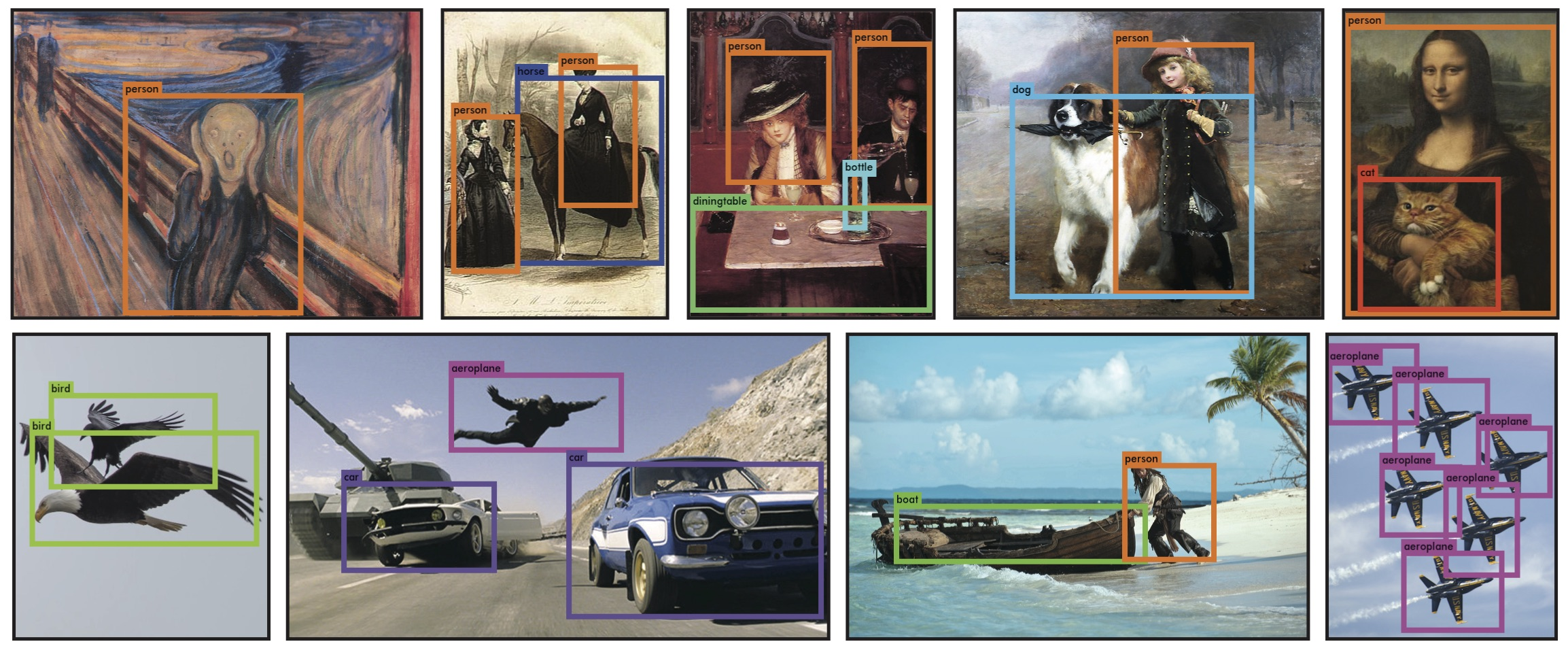
Detection: a box and a class for each object J. Redmon, S. Divvala, R. Girshick, A. Farhadi, “You Only Look Once: Unified, Real-Time Object Detection,” CVPR 2016, Fig. 6
Instance Segmentation Outlines Each Object
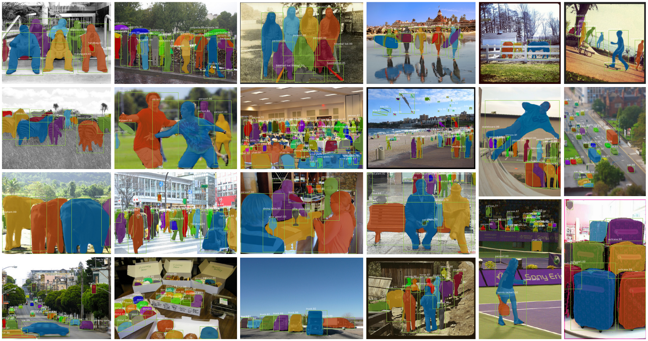
Instance segmentation: a box, a class, and a pixel mask for each object K. He, G. Gkioxari, P. Dollár, R. Girshick, “Mask R-CNN,” ICCV 2017, Fig. 5
Pose Estimation Locates Body Joints
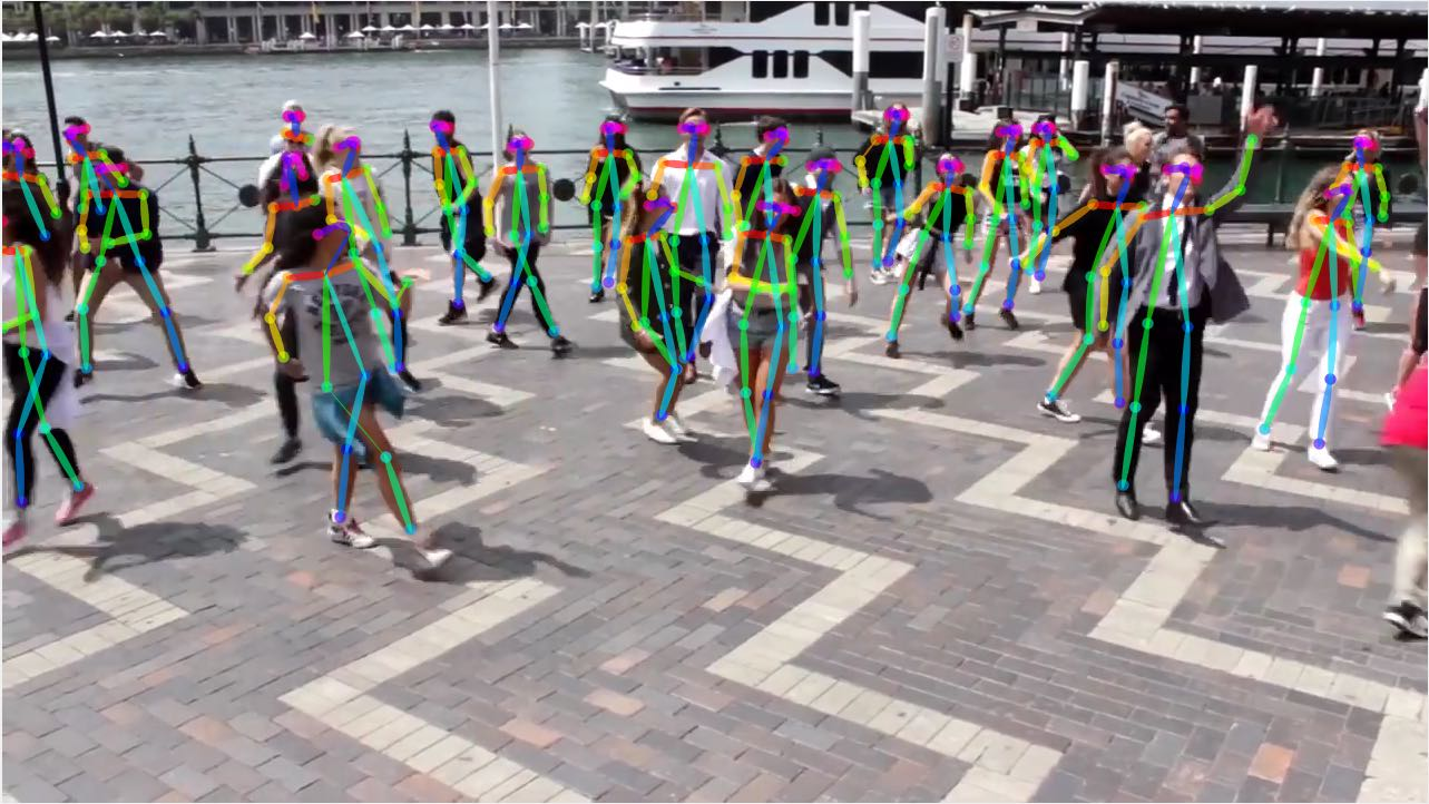
Pose estimation: the joints of every person, joined into skeletons Z. Cao, T. Simon, S.-E. Wei, Y. Sheikh, “Realtime Multi-Person 2D Pose Estimation Using Part Affinity Fields,” CVPR 2017, Fig. 1
Segmentation Classifies Every Pixel
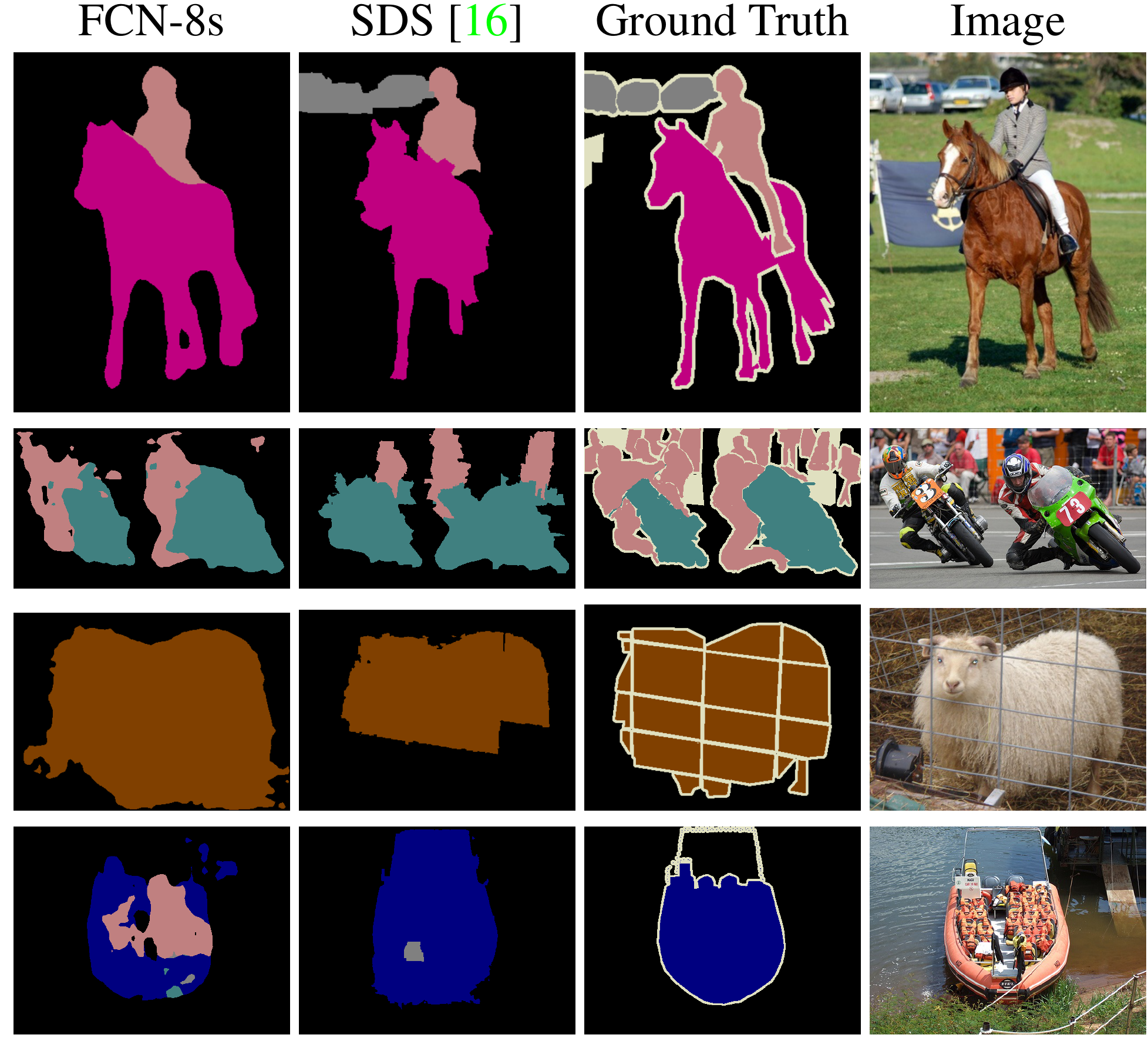
Semantic segmentation: a class for every pixel, against the ground truth; last row, life jackets labeled as people J. Long, E. Shelhamer, T. Darrell, “Fully Convolutional Networks for Semantic Segmentation,” CVPR 2015, Fig. 6
Convolutional Networks Segment Microscope Images
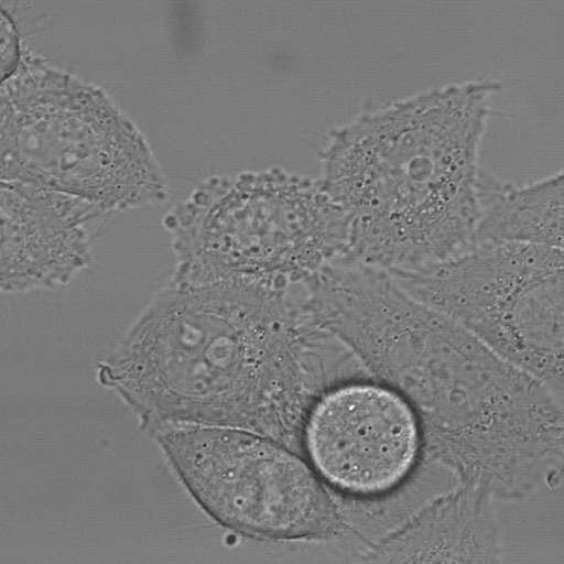
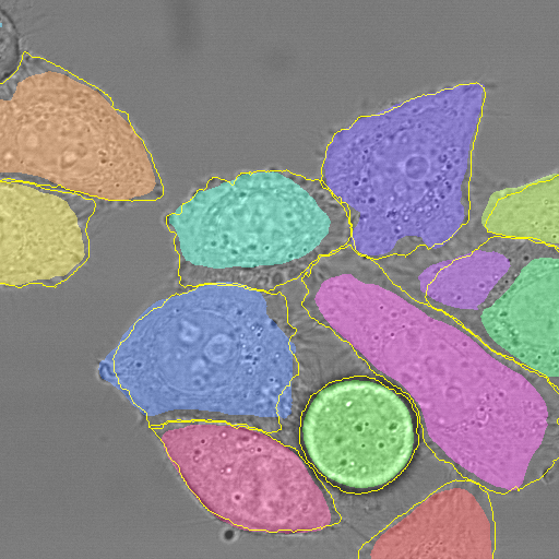
Cell segmentation: microscope image in, each cell outlined, from \(20\) partially annotated training images O. Ronneberger, P. Fischer, T. Brox, “U-Net: Convolutional Networks for Biomedical Image Segmentation,” MICCAI 2015, Fig. 4c, d
Style Transfer Repaints a Photograph in Another Image’s Style
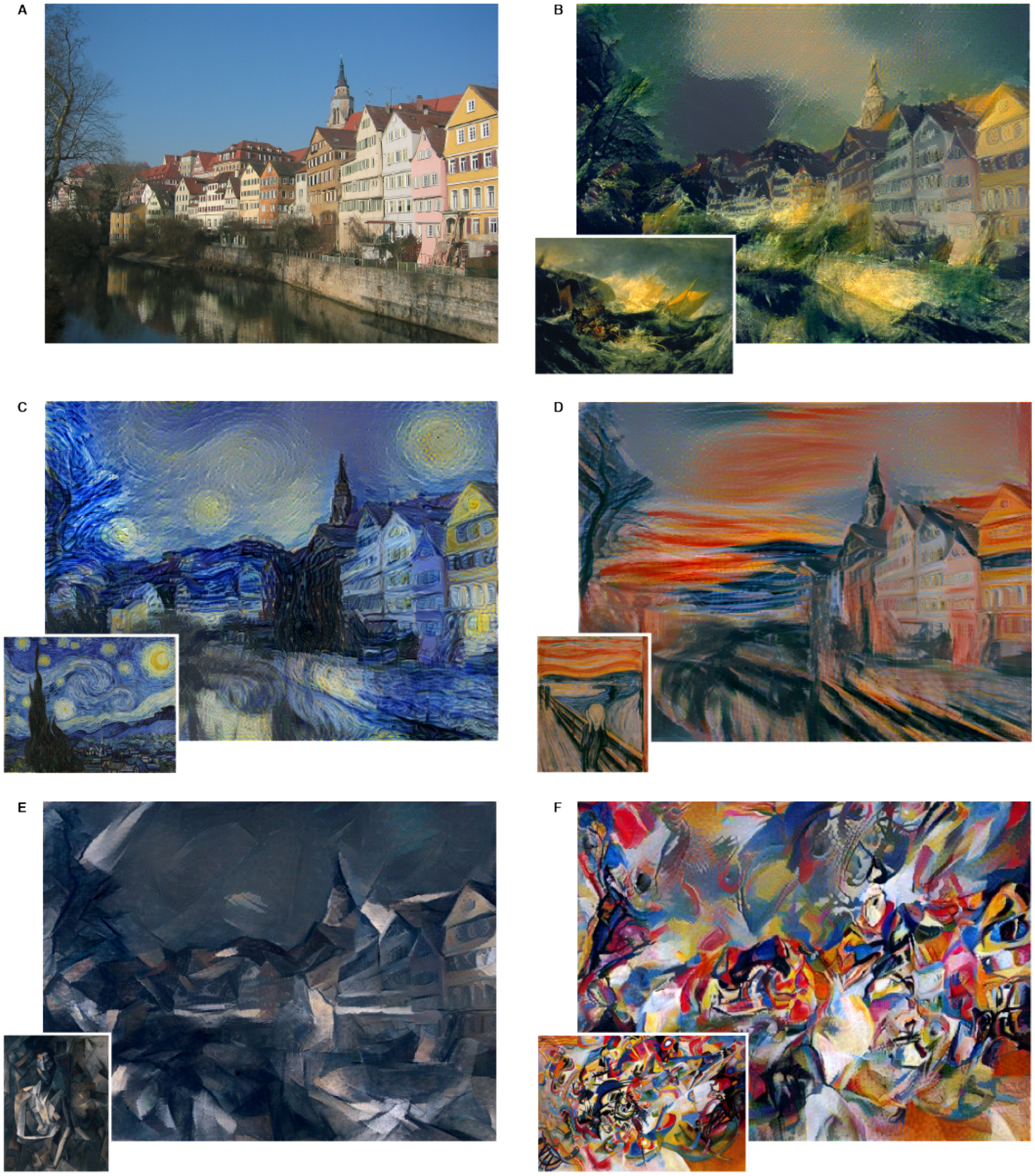
Style transfer: a photograph of Tübingen in the styles of Turner, van Gogh, Munch, Picasso, and Kandinsky L. A. Gatys, A. S. Ecker, M. Bethge, “A Neural Algorithm of Artistic Style,” arXiv 1508.06576, 2015, Fig. 2
Convolutional Networks Can Colorize Grayscale Images
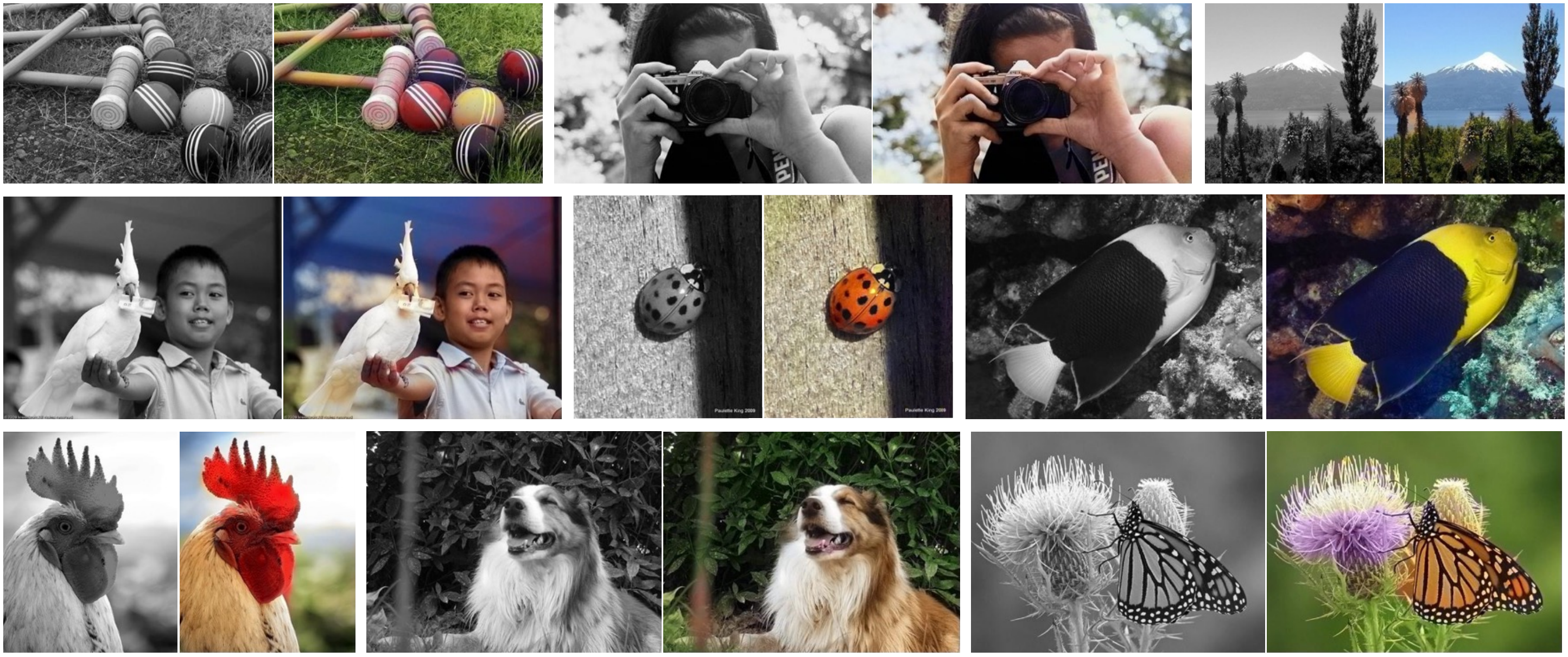
Colorization: a grayscale photograph in, a color photograph out R. Zhang, P. Isola, A. A. Efros, “Colorful Image Colorization,” ECCV 2016, Fig. 1
Super-Resolution Adds Detail to Low-Resolution Images
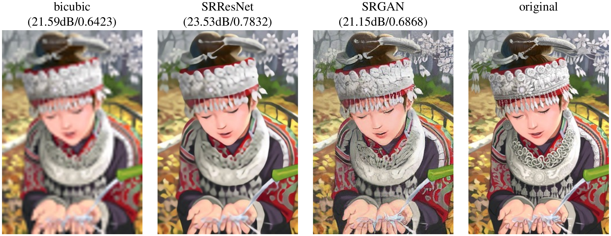
Super-resolution, \(4\times\): SRGAN looks sharpest and scores a lower PSNR than SRResNet C. Ledig et al., “Photo-Realistic Single Image Super-Resolution Using a Generative Adversarial Network,” CVPR 2017, Fig. 2
Captioning Describes an Image in Words
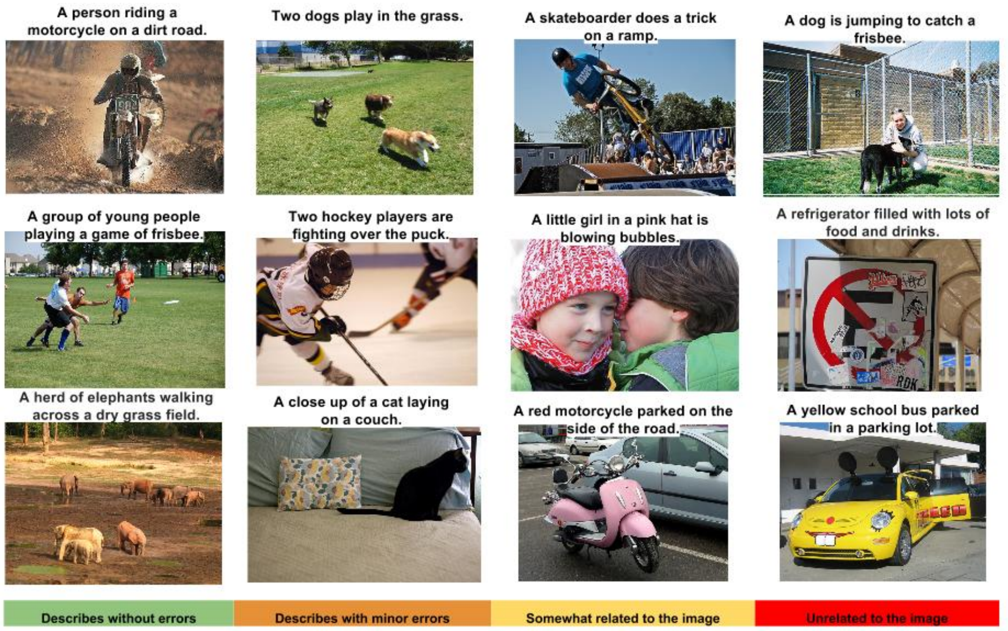
Captioning: generated captions, rated by people from without errors to unrelated to the image O. Vinyals, A. Toshev, S. Bengio, D. Erhan, “Show and Tell: A Neural Image Caption Generator,” CVPR 2015, Fig. 5
Attention Maps Link Each Word to an Image Region
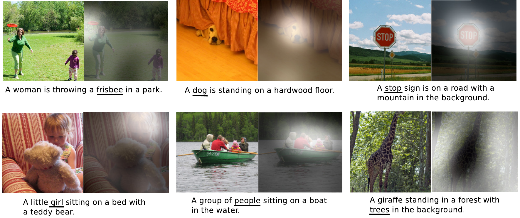
Attention: the bright region is where the network looked for the underlined word K. Xu et al., “Show, Attend and Tell: Neural Image Caption Generation with Visual Attention,” ICML 2015, Fig. 3
Generative Networks Synthesize Realistic Faces
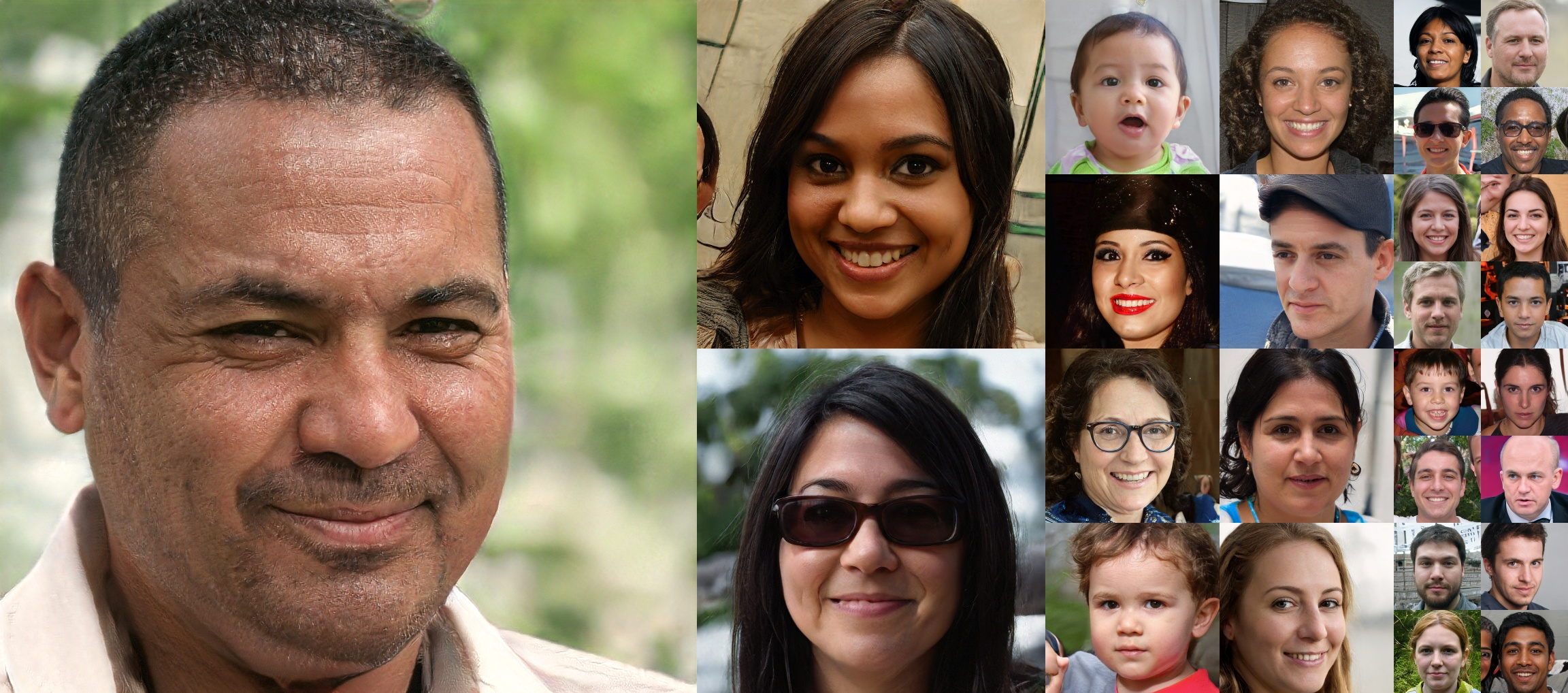
Generation: faces produced by a network, uncurated T. Karras, S. Laine, T. Aila, “A Style-Based Generator Architecture for Generative Adversarial Networks,” CVPR 2019, Fig. 2 (top)
Convolution Assumes Local Patterns at Any Grid Position
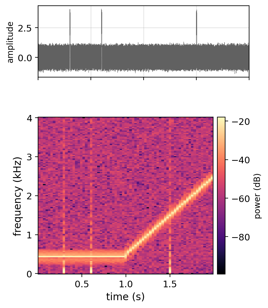
Spectrogram: an audio signal as a grid of time by frequency
- Tone, chirp, click: locally a horizontal, rising, and vertical line
- Along time, the same pattern at any position
- Along frequency, a shift changes the pitch: the condition holds in part
Signal: \(440\) Hz tone, chirp from \(500\) to \(2{,}500\) Hz, three clicks
Game screens: Atari frames in, the next action out (Mnih et al. 2013)
One dimension: raw signals and sequences, such as audio and ECG
Three dimensions: video, over time, height, and width
No order: tabular data, whose column order is arbitrary
- A kernel over columns depends on that arbitrary order
An LTI Filter Computes Each Output From a Local Window
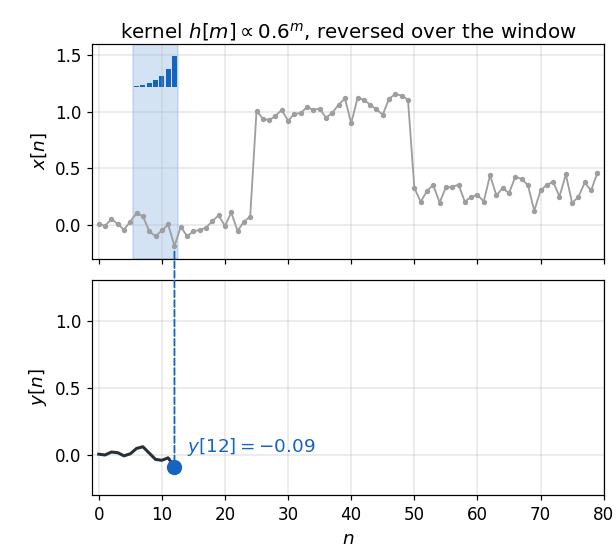
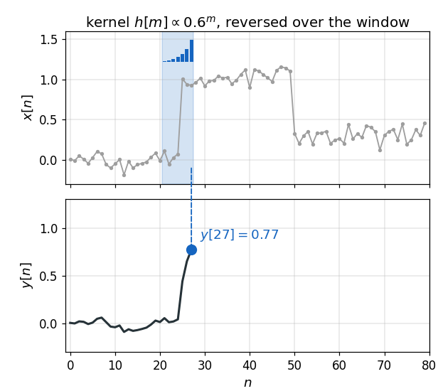
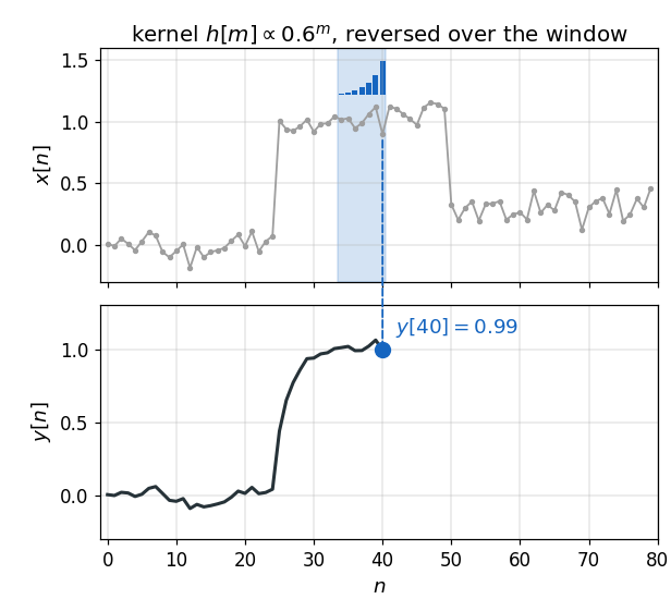
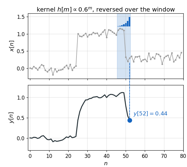
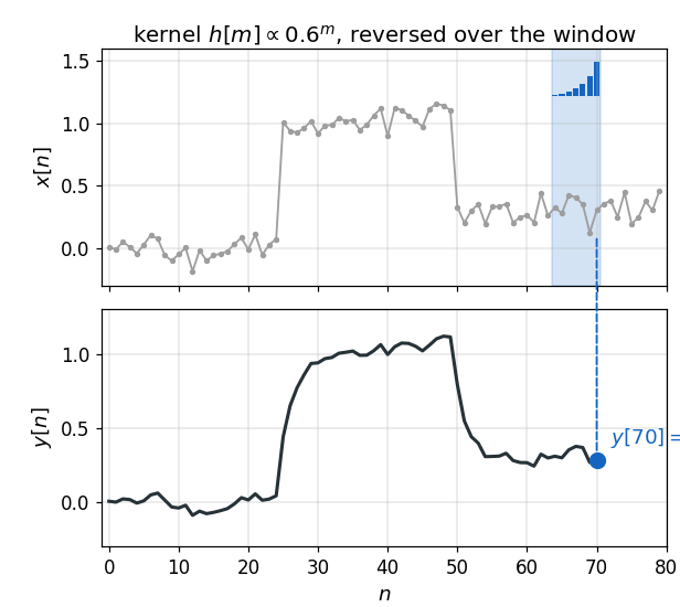
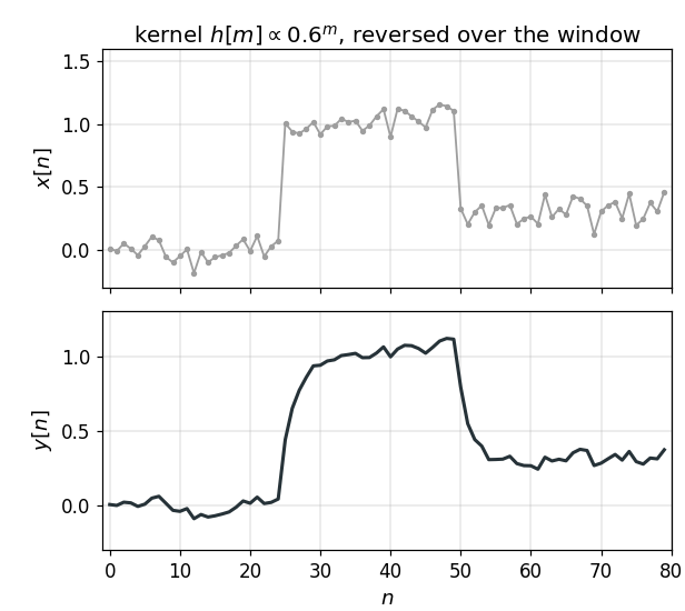
Low-pass filter: a truncated exponential moving average, \(h[m] \propto 0.6^m\)
Convolution, signal processing \[y[n] = \sum_{m} h[m]\, x[n - m]\]
Impulse response \(h\): the output for a unit impulse
Time invariance: one \(h\) for every \(n\)
Kernel: the weights \(h[m]\), here \(7\) of them
Local: each output depends on the \(7\) samples under the kernel only
A Learned Kernel Is a Learned Filter
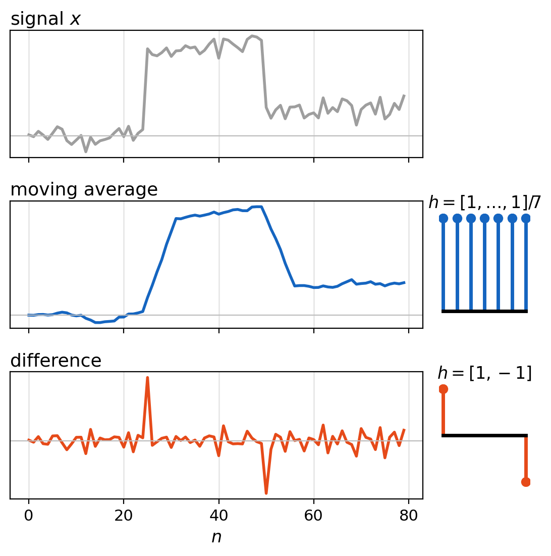
Moving average, \(h = [1, \ldots, 1]/7\), low-pass
- Noise reduced
- Slow trend kept
Difference, \(h = [1, -1]\), step detector
- Near \(0\) on flat segments
- A spike at each step
- Sign: step up or step down
Same sum, different \(h\)
In a convolutional layer: the kernel is learned
Correlation Is Convolution With the Kernel Reversed
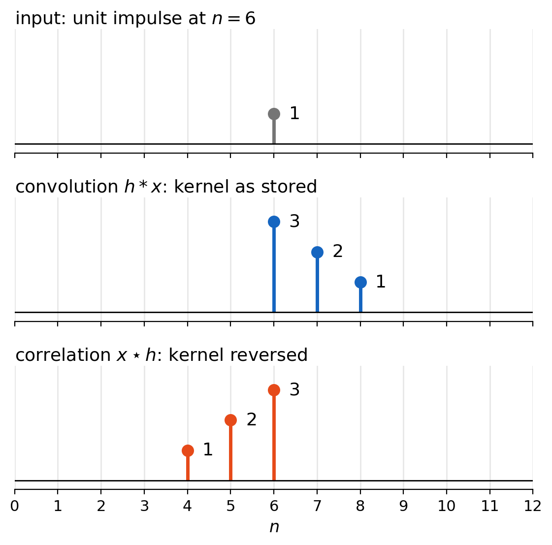
Convolution: \(\;(x * h)[n] = \sum_m h[m]\, x[n - m]\)
Correlation: \(\;(x \star h)[n] = \sum_m h[m]\, x[n + m]\)
At an impulse
- Convolution: the kernel, \(3, 2, 1\)
- Correlation: the kernel reversed, \(1, 2, 3\)
nn.Conv2d: correlation, plus a bias
- Kernel written \(w\)
Learned kernel
- Convolution with \(h\) = correlation with \(h\) reversed
- Both define the same set of layers
2D Correlation Computes Each Output From a Local Patch
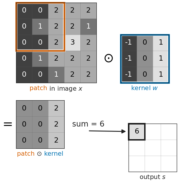
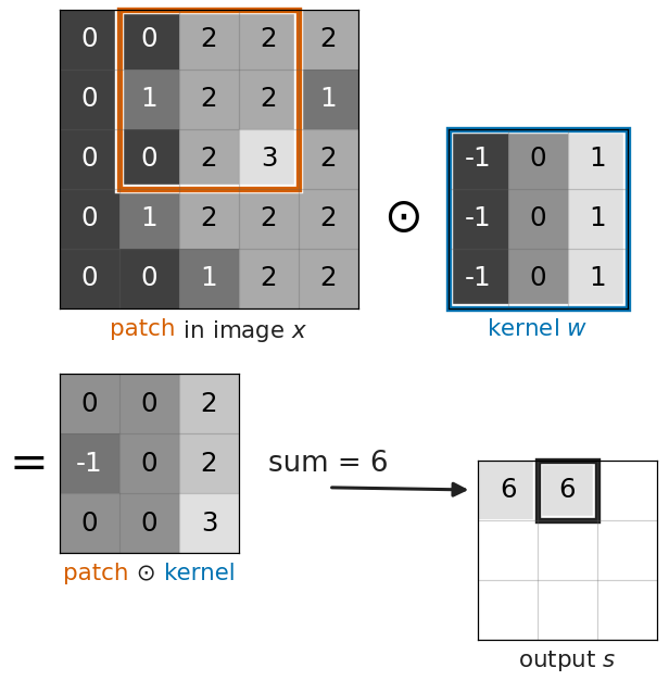
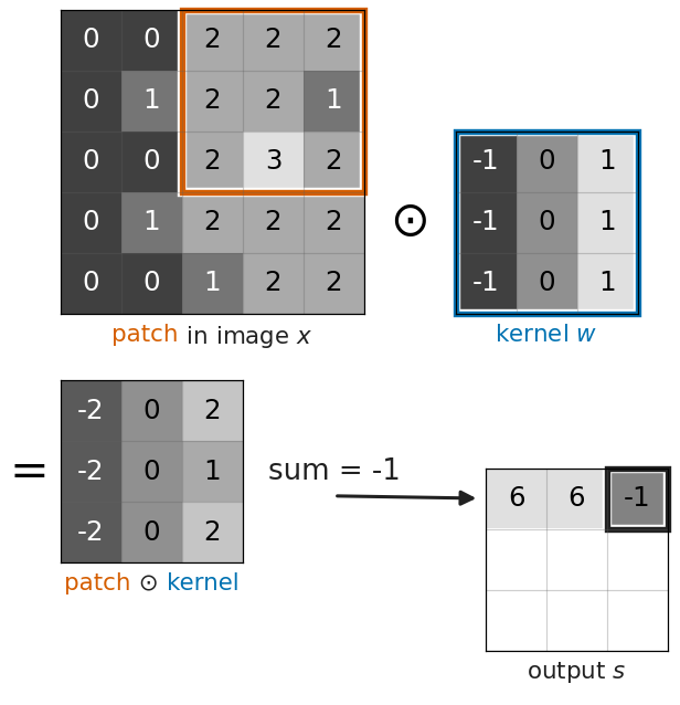
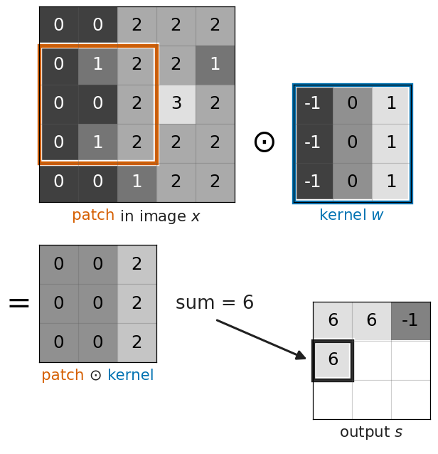
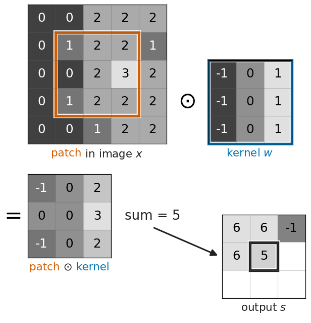
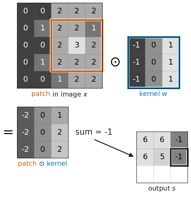
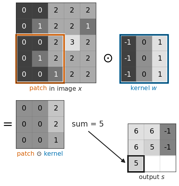
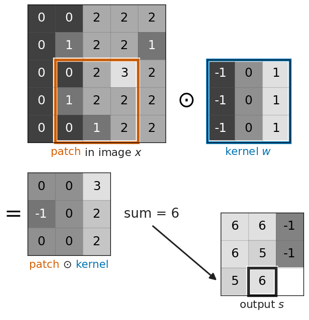
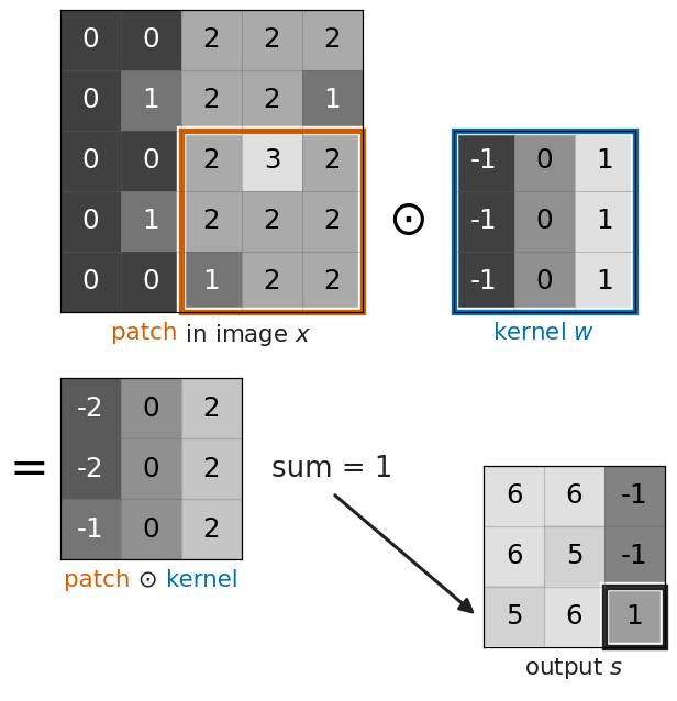
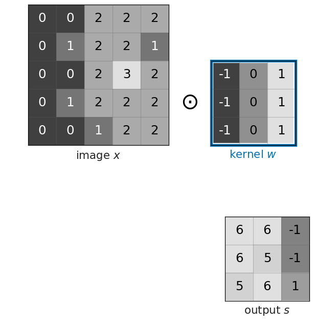
Correlation in 2D \[s[i, j] = \sum_{m=0}^{2}\sum_{n=0}^{2} w[m, n]\, x[i + m,\, j + n]\]
From one dimension
- Signal \(x[n]\): image \(x[i, j]\)
- \(h\): kernel \(w\)
- \(y\): map \(s\)
Local: each output depends on one \(3 \times 3\) patch only
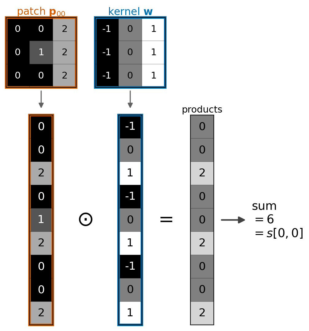
Example: \(+1\) right column, \(-1\) left column
- \(s[0, 0] = 6\): the patch brightens left to right
- \(s[0, 2] = -1\): the patch darkens left to right
Each Output Is a Dense Unit’s Inner Product on One Patch
Dense unit, one image: \(s = \mathbf{w}^T\mathbf{x} + b\)
- \(784\) weights, one per pixel
Convolutional unit, one patch: \(s[i, j] = \mathbf{w}^T\mathbf{p}_{ij} + b\)
- \(\mathbf{p}_{ij}\): the \(3 \times 3\) patch at \((i, j)\), flattened to \(9\) values
- Kernel \(\mathbf{w}\): \(9\) weights, the same at every \((i, j)\)
Same computation: a dense unit on \(9\) inputs, repeated at every position
Patches Aligned With the Kernel Give Larger Responses
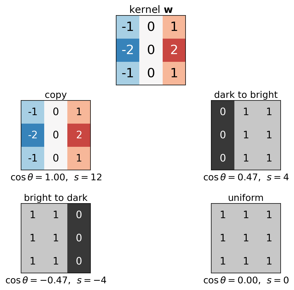
\[s = \mathbf{w}^T\mathbf{p} = \underbrace{\|\mathbf{w}\|}_{\text{kernel}}\;\underbrace{\|\mathbf{p}\|}_{\text{patch norm}}\;\underbrace{\cos\theta}_{\text{alignment}}\]
- Alignment: at most \(1\), reached at \(\mathbf{p} = c\,\mathbf{w}\), \(c > 0\) (Cauchy–Schwarz)
- Patch norm: scales \(s\), leaves \(\cos\theta\) unchanged
- Uniform patch: \(s = 0\), since the kernel’s weights sum to \(0\)
Kernel in the figure: vertical edge, dark to bright
Matched Kernels Detect Weak Patterns in Pixel Noise
Per pixel
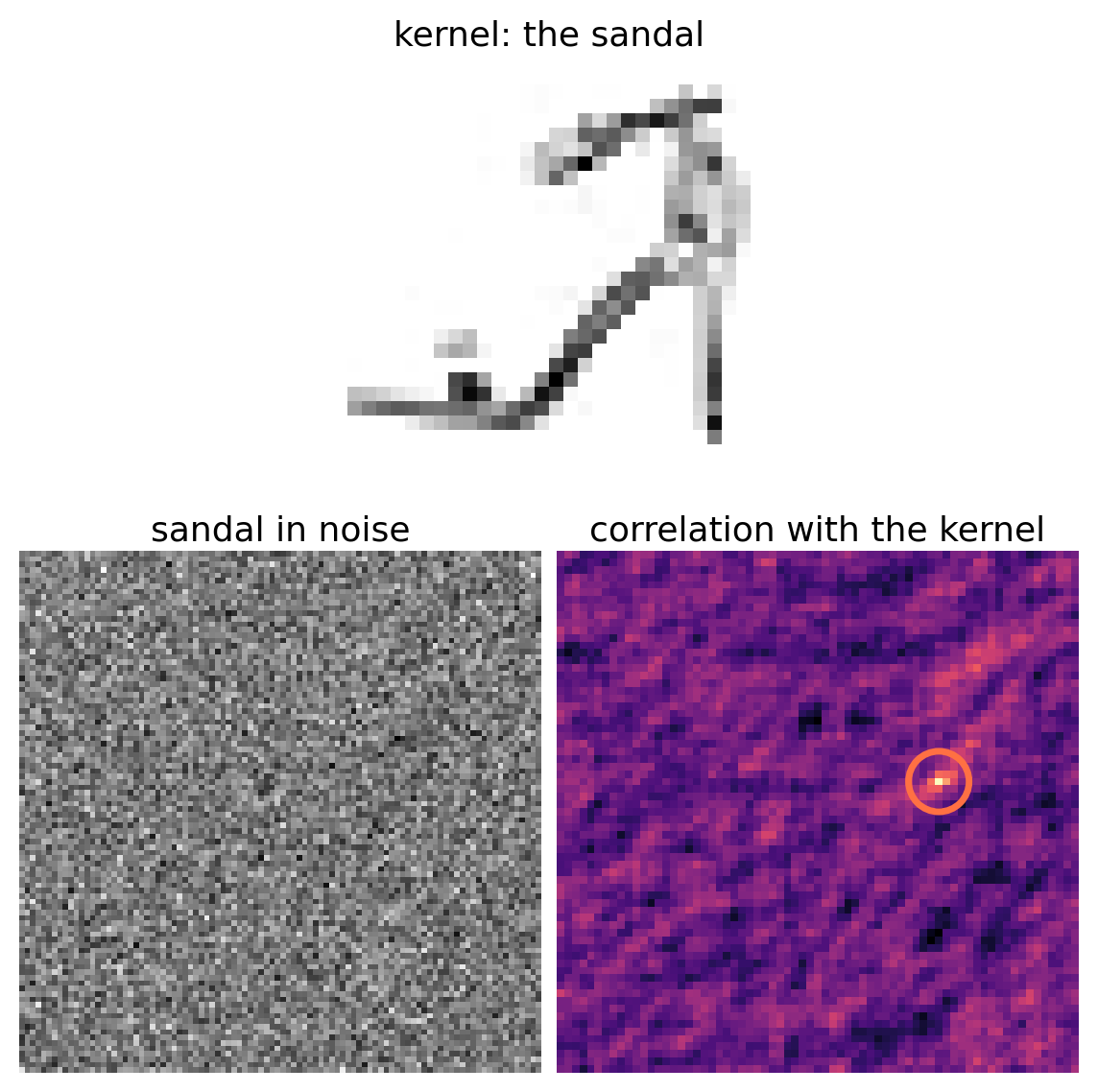
- Sandal: root-mean-square 0.11
- Noise: standard deviation \(0.35\)
Kernel output, \(784\) pixels
Unit-norm kernel: output noise \(\sigma = 0.35\)
Peak 2.88, noise standard deviation \(0.35\)
8 standard deviations
Gain \(\sqrt{784} = 28\) over one pixel
Largest response: row 30, column 50, where the sandal was placed
A Local Kernel Reduces an Image to Its Outlines
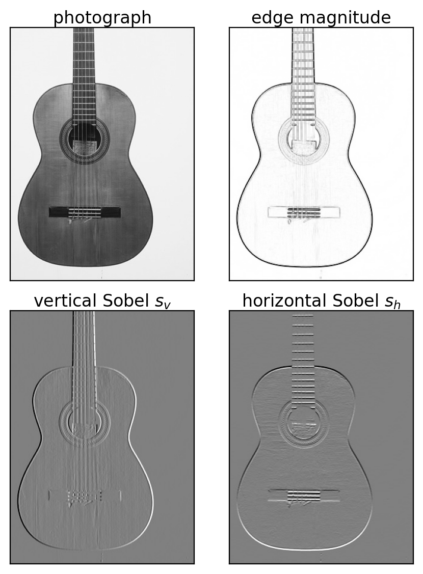
Sobel kernels: a gradient estimate, built by design
\[\begin{bmatrix} -1 & 0 & 1 \\ -2 & 0 & 2 \\ -1 & 0 & 1 \end{bmatrix} = \begin{bmatrix} 1 \\ 2 \\ 1 \end{bmatrix} \begin{bmatrix} -1 & 0 & 1 \end{bmatrix}\]
- Central difference \([-1, 0, 1]\) across the edge
- Smoothing \([1, 2, 1]\) along it, against noise
- Horizontal kernel: the transpose
Edge magnitude: \(\sqrt{s_v^2 + s_h^2}\)
I. Sobel and G. Feldman, “An Isotropic 3×3 Image Gradient Operator,” Stanford AI Project, 1968. Photograph: guitar by Manuel Ramírez, 1912, The Metropolitan Museum of Art (CC0)
Convolutional Networks Learn Simple Patterns in Early Layers
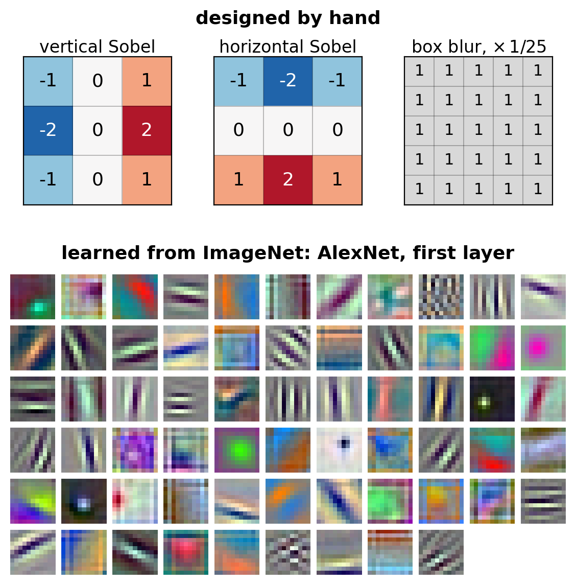
AlexNet: a convolutional network, \(5\) convolutional layers, then \(3\) dense layers, trained on ImageNet
First layer, shown: \(64\) kernels, weights fit by gradient descent
Learned
- Oriented edges and stripes at many angles
- Color patches: weights that differ across the three channels
Operation: correlation, as with the Sobel kernels
torchvision AlexNet, ImageNet weights: \(64\) kernels, the one-GPU network of A. Krizhevsky, arXiv 1404.5997, 2014 (the 2012 network has \(96\))
A Convolutional Layer Is a Dense Layer With Sparse, Shared Weights
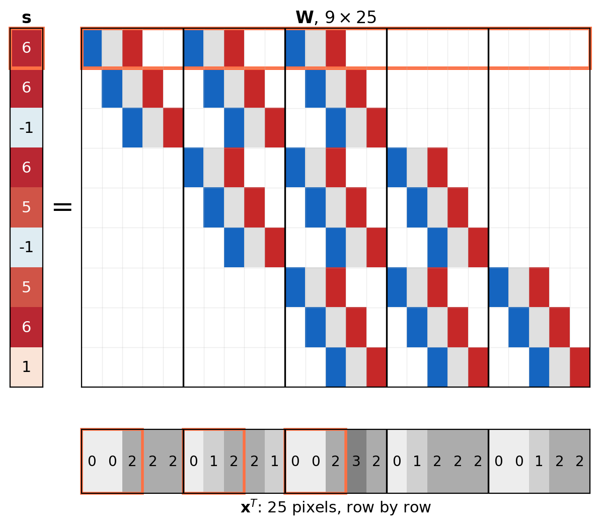
\(\mathbf{s} = \mathbf{W}\mathbf{x}\), the \(5 \times 5\) example flattened row by row
Row \((i, j)\) of \(\mathbf{W}\): the kernel’s \(9\) values at the columns of patch \((i, j)\)
Sparse: zero outside the patch, \(81\) of \(225\) entries on a patch, \(54\) of them nonzero
Shared: the same \(9\) values in every row
Backward pass: \(\partial\ell/\partial\mathbf{x} = \mathbf{W}^T\,\partial\ell/\partial\mathbf{s}\)
The Number of Convolutional Weights Does Not Depend on Input Size
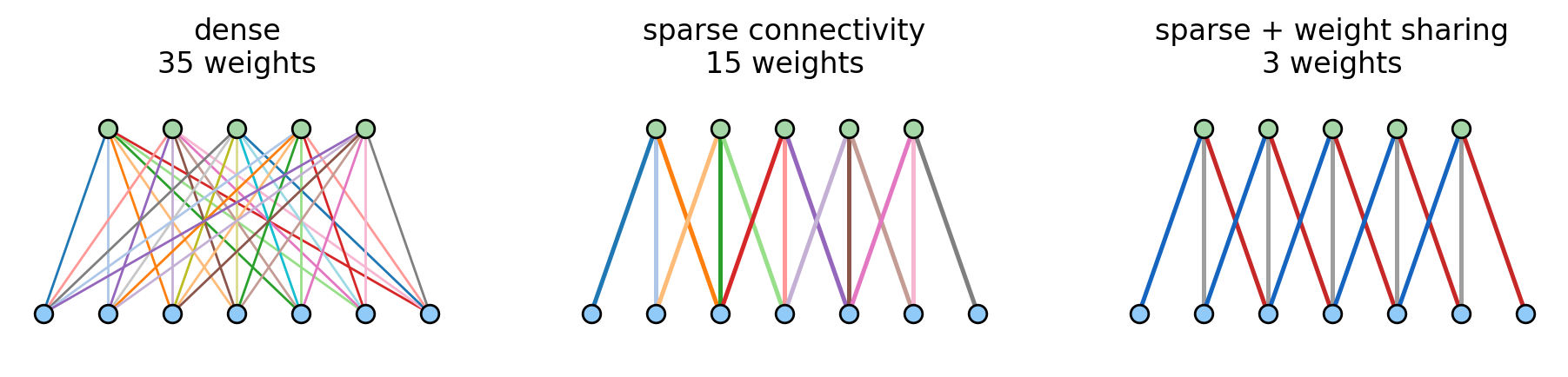
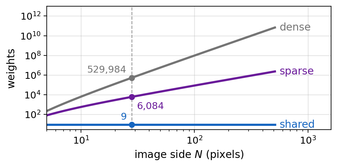
Number of weights, \(N \times N\) input, \(3 \times 3\) kernel
- Dense: \((N-2)^2 N^2\)
- Sparse connectivity: \(9\,(N-2)^2\)
- Sparse + weight sharing: \(9\)
At \(N = 28\): \(529{,}984\), \(6{,}084\), \(9\)
Multiplications: \(9\,(N-2)^2\), with or without sharing
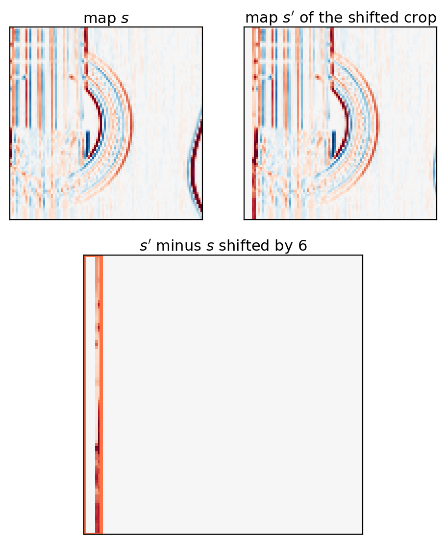
Convolution Is Translation Equivariant
Input shifted right by \(t\), zero fill: \(x'[i, j] = x[i, j - t]\)
\[s'[i, j] = \sum_{m, n} w[m, n]\, x[i + m,\, j - t + n] = s[i, j - t]\]
Equivariant: input shifted by \(t\), output shifted by \(t\)
Condition: \(w[m, n]\) independent of \((i, j)\)
- Different weights at each position: not equivariant
Borders: equality for \(j \ge t\)
Signal-processing name: shift invariance of the system
Kernels Spanning the Color Channels Detect Edges Between Colors
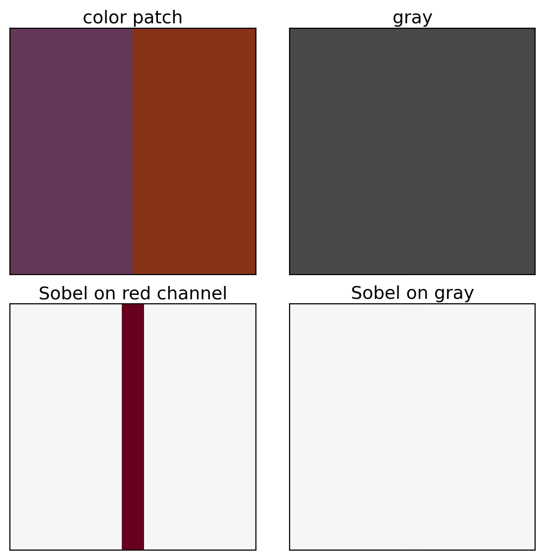
Gray value: \(0.299R + 0.587G + 0.114B\)
Purple sky, orange horizon
- Different colors
- Gray value 0.29 for each
Sobel on the red channel alone: edge detected
Sobel on gray: \(s = 0\) at the boundary
A Kernel Sums Over Every Input Channel
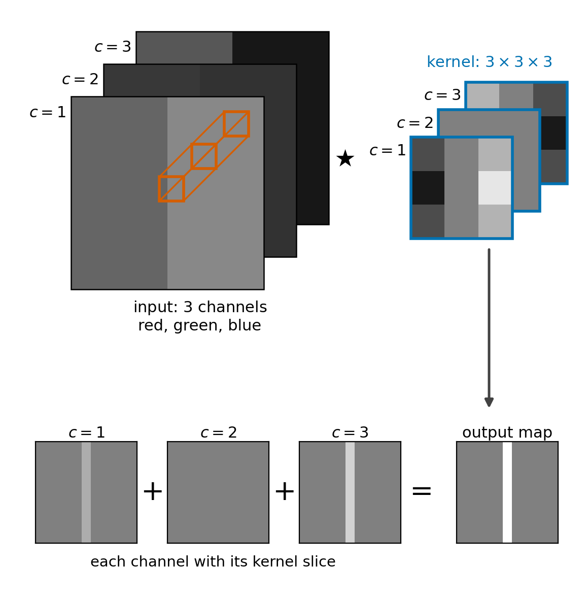
Input: \(C_{\text{in}}\) channels
- Color image: red, green, blue, \(C_{\text{in}} = 3\)
Kernel: \(C_{\text{in}} \times k \times k\) weights, one \(k \times k\) slice per channel
- Depth \(C_{\text{in}}\): slides over height and width only
- Equal to \(C_{\text{in}}\) single-channel convolutions, summed
\[s[i, j] = \sum_{c=1}^{C_{\text{in}}} \sum_{m, n} w[c, m, n]\; x[c, i + m,\, j + n] + b\]
- Inner product over \(C_{\text{in}} k^2\) values
- One output map
Example: purple against orange, equal gray
- Red slice: vertical-edge kernel
- Blue slice: its negative
- Peak response 1.55 at the boundary
\(C_{\text{out}}\) Kernels Give \(C_{\text{out}}\) Output Channels
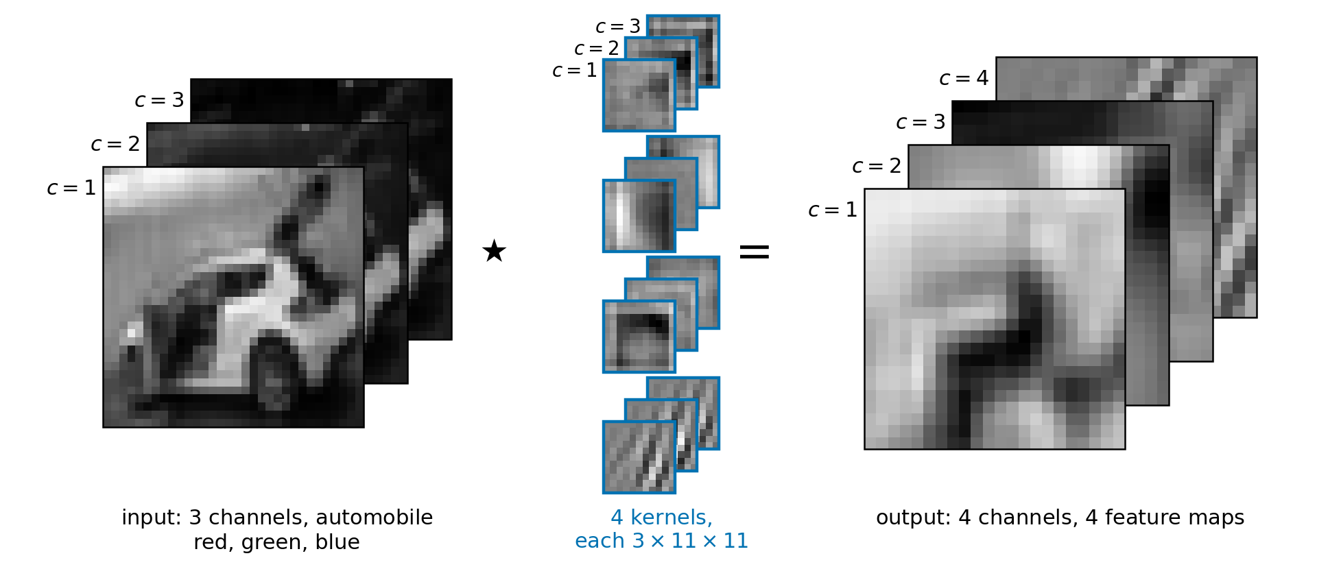
Weights: \(C_{\text{out}} \times C_{\text{in}} \times k \times k\), one bias per output channel
Output: \(C_{\text{out}}\) maps, a \(C_{\text{out}}\)-channel image
Kernels shown: \(4\) of the \(64\) first-layer kernels of torchvision’s AlexNet, on a CIFAR-10 image
Feature Maps Are the Next Layer’s Input Channels
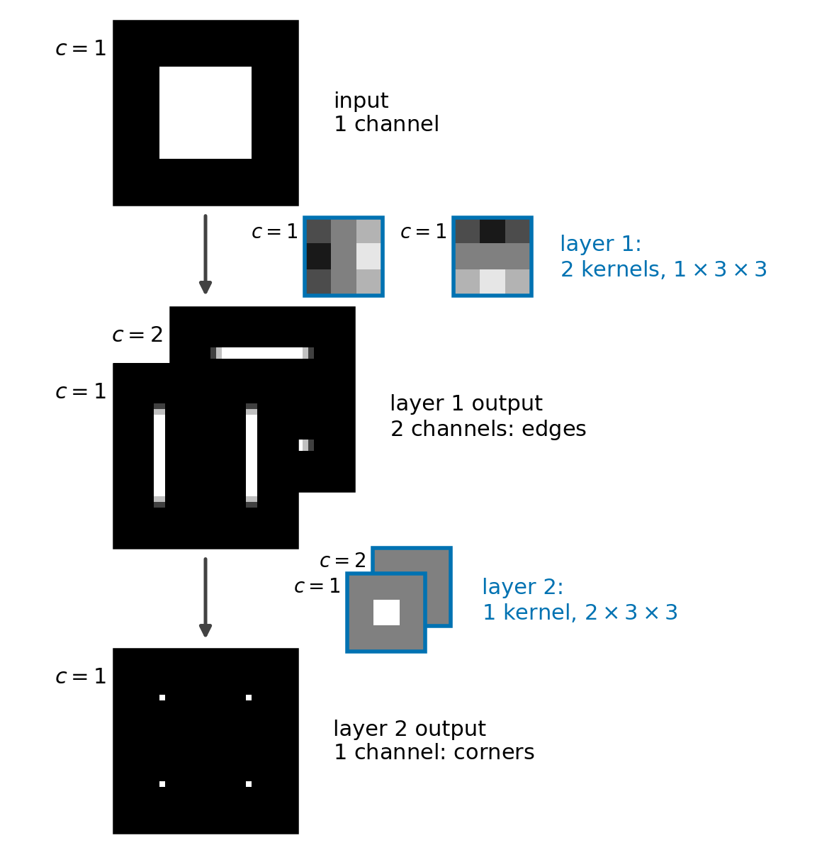
Layer 1: \(2\) kernels, \(2\) output channels
- \(|\)Sobel\(|\) responses scaled to at most \(1\): vertical edges, horizontal edges
Layer 2, set by hand: kernel of shape \(2 \times 3 \times 3\), one slice per edge channel
- Center weight \(1\) in each slice, bias \(-1\), ReLU
- Positive only where both edge maps are nonzero: the corners
Convolutional Layers Do Far More Computation per Parameter Than Dense Layers
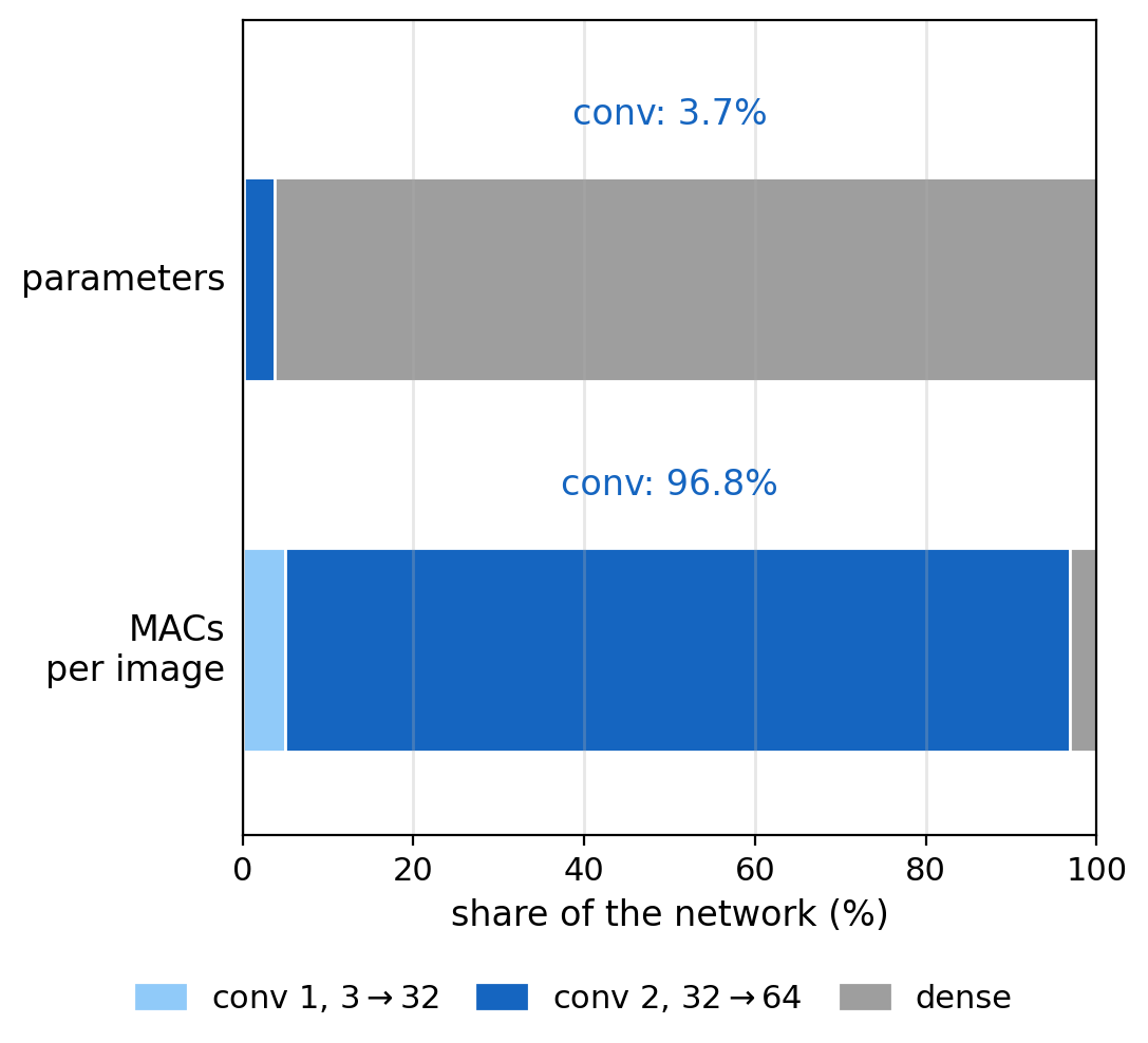
Network, \(32 \times 32 \times 3\) input
- Conv, \(3\) to \(32\) channels, \(3 \times 3\): \(896\) parameters
- Conv, \(32\) to \(64\) channels: \(18{,}496\)
- Dense, \(50{,}176\) inputs to \(10\) outputs: \(501{,}770\)
MACs per layer: weights × output positions
- Conv 2: \(18{,}432\) weights, \(28 \times 28\) positions, \(14{,}450{,}688\)
MACs per weight: \(784\) in conv 2, \(1\) in the dense layer
A Unit’s Input Region Grows Linearly With Depth
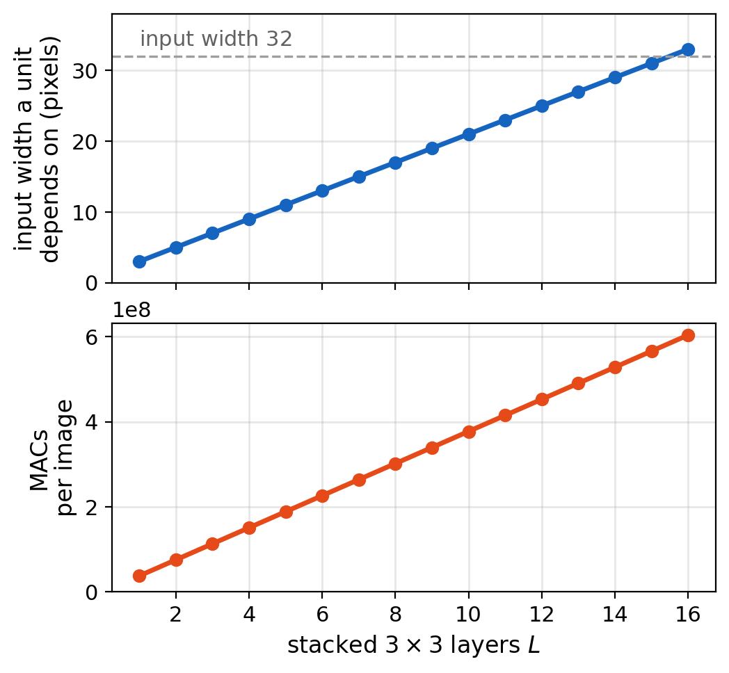
One \(3 \times 3\) layer: each unit depends on a \(3 \times 3\) input region
\(L\) layers: \((2L + 1) \times (2L + 1)\)
- \(L = 3\): \(7 \times 7\)
- \(L = 16\): \(33 \times 33\), the whole \(32 \times 32\) input
Maps kept at \(32 \times 32\), \(64\) channels: the same cost at every layer
Cost: 0.6 billion MACs per image for \(16\) layers, linear in \(L\)